twistpy.polarization.DispersionAnalysis

class DispersionAnalysis(traN: Optional[Trace] = None, traE: Optional[Trace] = None, traZ: Optional[Trace] = None, rotN: Optional[Trace] = None, rotE: Optional[Trace] = None, rotZ: Optional[Trace] = None, fmin: float = 1.0, fmax: float = 20.0, octaves: float = 0.5, window: dict = {'number_of_periods': 1, 'overlap': 0.0}, scaling_velocity: float = 1.0, svm: Optional[SupportVectorMachine] = None, verbose: bool = True)

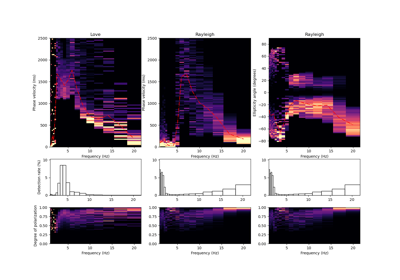
Single-station six-component surface wave dispersion estimation for Love and Rayleigh waves.

Under the hood, the DispersionAnalysis class runs a TimeDomainAnalysis6C. The data is filtered to different frequency bands of interest, and the wave parameters are estimated at each frequency independently.

Parameters

traNTrace

North component of translation

traETrace

East component of translation

traZTrace

Vertical component of translation (positive downwards!)

rotNTrace

North component of rotation

rotETrace

East component of rotation

rotZTrace

Vertical component of rotation (right-handed, pointing downwards!)

fminfloat

Minimum frequency to be considered in the analysis (in Hz)

fmaxfloat

Maximum frequency to be considered in the analysis (in Hz)

octavesfloat

Width of the frequency band used for bandpass filtering in octaves

windowdict

Window parameters defined as:

window = {‘number_of_periods’: float, ‘overlap’: float}

Overlap should be on the interval 0 (no overlap between subsequent time windows) and 1 (complete overlap, window is moved by 1 sample only). The window is frequency dependent and extends over number_of_periods times the dominant period at the current frequency band

scaling_velocityfloat, default=1.

Scaling velocity (in m/s) to ensure numerical stability. The scaling velocity is applied to the translational data only (amplitudes are divided by scaling velocity) and ensures that both translation and rotation amplitudes are on the same order of magnitude and dimensionless. Ideally, v_scal is close to the S-Wave velocity at the receiver. After applying the scaling velocity, translation and rotation signals amplitudes should be similar. svm

verbosebool, default=True

Run in verbose mode.

Attributes

parameterslist of dict

List containing the estimated surface wave parameters at each frequency. The parameters for each frequency are saved in a dictionary with the following keys:

‘xi’: Rayleigh wave ellipticity angle (degrees)

‘phi_r’: Rayleigh wave back-azimuth (degrees)

‘c_r’: Rayleigh wave phase-velocity (m/s)

‘phi_l’: Love wave back azimuth (degrees)

‘c_l’: Love wave phase velocity (m/s)

‘wave_types’: Wave type classification labels

‘dop’: Degree of polarization

fnumpy.ndarray of float

Frequency vector for parameters.

Methods

plot([nbins, velocity_range, quantiles, ...])	Plot estimated Love- and Rayleigh-wave dispersion curves and Rayleigh wave ellipticity angle.
plot_baz([freq, nbins, show])	Plot the back-azimuth of Love and Rayleigh wave sources as a polar plot.
save(name)	Save the current DispersionAnalysis object to a file on the disk in the current working directory.

Examples using twistpy.polarization.DispersionAnalysis

Six-component dispersion analysis

Six-component dispersion analysis