6-C Wave parameter estimation: gulf of alaska earthquake

This tutorial will teach you how to use TwistPy to process six component seismic data as recorded by collocated translational and rotational seismometers. The data used in this tutorial was recorded at the large ring laser observatory ROMY in Furstenfeldbruck, Germany after the January, 23rd 2018 M7.8 gulf of Alaska earthquake (Occurence Time: 2018-01-23 09:31:40 UTC).

from obspy import read

from twistpy.polarization import TimeFrequencyAnalysis6C, EstimatorConfiguration

We start by reading in the 6DOF data and apply some basic pre-processing to it using standard ObsPy functionality. To ensure that the amplitudes of all six time series are on the same order of magnitude and have the same unit, we apply a scaling velocity to the translational components:

data = read("../example_data/ROMY_gulf_of_alaska_teleseism.mseed")
scaling_velocity = 4500.0

for n, trace in enumerate(data):
    trace.detrend("spline", order=5, dspline=100)
    trace.trim(starttime=trace.stats.starttime, endtime=trace.stats.endtime - 4500)
    trace.taper(0.2)
    if n < 3:
        trace.data /= scaling_velocity

Now we are ready to set up the 6DOF polarization analysis problem. The spectral matrices from which the polarization attributes are estimated are computed in a time-frequency window. We choose the window to be frequency-dependent and extend over 1 period (1/f) in the time direction and over 0.01 Hz in the frequency direction:

window = {"number_of_periods": 1, "frequency_extent": 0.01}

Now we are ready to set up the 6DOF polarization analysis problem. We want to perform the analysis in the time-frequency domain, so we set up a TimeFrequencyAnalysis6C object and feed it our data and the polarization analysis window. Additionally, we restrict the analysis to the frequency range between 0.01 and 0.15 Hz, where we expect surface waves to dominate. To reduce the computational effort, we only compute wave paramters at every 20th sample in time and in frequency:

analysis = TimeFrequencyAnalysis6C(
    traN=data[0],
    traE=data[1],
    traZ=data[2],
    rotN=data[3],
    rotE=data[4],
    rotZ=data[5],
    window=window,
    dsfacf=20,
    dsfact=20,
    frange=[0.01, 0.15],
)

Computing covariance matrices...
Covariance matrices computed!

Now we set up an EstimaatorConfiguration, specifying for which wave types we want to estimate wave parameters (in this example only Rayleigh waves), what kind of estimator we want to use, and the range of wave parameters that are tested.

est = EstimatorConfiguration(
    wave_types=["R"],
    method="DOT",
    scaling_velocity=scaling_velocity,
    use_ml_classification=False,
    vr=[3000, 4000, 100],
    xi=[-90, 90, 2],
    phi=[150, 210, 1],
    eigenvector=0,
)

Let’s start the analysis!

analysis.polarization_analysis(estimator_configuration=est)

Computing wave parameters...
Estimating wave parameters for R-Waves...
Done!

Once the wave parameters are computed, we can access them as a dictionary obtained from the attribute wave_parameters.

print(analysis.wave_parameters)

{'P': {'vp': None, 'vp_to_vs': None, 'theta': None, 'phi': None, 'lh': None}, 'SV': {'vp': None, 'vp_to_vs': None, 'theta': None, 'phi': None, 'lh': None}, 'SH': {'vs': None, 'theta': None, 'phi': None, 'lh': None}, 'R': {'vr': array([[4000, 4000, 4000, ..., 4000, 4000, 4000],
       [3000, 3000, 3000, ..., 3900, 3800, 3900],
       [4000, 4000, 3000, ..., 4000, 4000, 4000],
       ...,
       [3500, 3000, 3000, ..., 3000, 3000, 3000],
       [3400, 3000, 3000, ..., 3000, 3000, 3000],
       [3500, 3000, 3000, ..., 3000, 3000, 4000]]), 'phi': array([[210, 210, 210, ..., 210, 210, 210],
       [150, 150, 150, ..., 174, 169, 157],
       [152, 157, 187, ..., 168, 162, 154],
       ...,
       [150, 150, 196, ..., 150, 151, 210],
       [150, 150, 193, ..., 150, 151, 210],
       [163, 150, 187, ..., 156, 154, 210]]), 'xi': array([[-52, -50, -50, ..., -54, -54, -54],
       [-32, -24, -12, ..., -20, -28, -30],
       [-72, -68, -28, ..., -76, -72, -68],
       ...,
       [-56, -16, -22, ..., -76, -84, -76],
       [-56, -12, -20, ..., -76, -84, -70],
       [-54, -10, -22, ..., -74, -82, -62]]), 'lh': array([[0.60708311, 0.58872218, 0.50825084, ..., 0.69386143, 0.69218305,
        0.6920553 ],
       [0.47834236, 0.45748968, 0.41683573, ..., 0.54862892, 0.54767244,
        0.52601953],
       [0.57445563, 0.59898155, 0.53772858, ..., 0.57399101, 0.58474929,
        0.58262612],
       ...,
       [0.53654438, 0.38803749, 0.35921063, ..., 0.46655726, 0.43623477,
        0.40777024],
       [0.5576458 , 0.37849171, 0.34852738, ..., 0.41553094, 0.45177927,
        0.43573335],
       [0.53368348, 0.37949115, 0.33713734, ..., 0.37192061, 0.46599798,
        0.45128402]])}, 'L': {'vl': None, 'phi': None, 'lh': None}}

To directly extract the Rayleigh wave parameters, we can access them in the following way (here we extract the Rayleigh wave propagation azimuth). With the corresponding time and frequency vectors.

azi_rayleigh = analysis.wave_parameters["R"]["phi"]
f = analysis.f_pol
t = analysis.t_pol

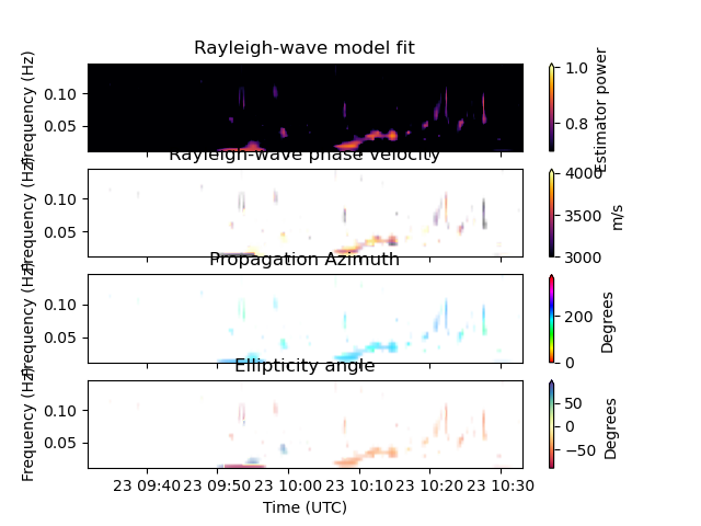
You can either plot the estimated parameters yourself or make use of the implemented plotting routines, where lh_min and lh_max determine the estimator power range for which the parameters are plotted. For the ‘DOT’ method that we used here, this corresponds to a simple likelihood, meaning that we only want to plot the results at time-frequency pixels where the Rayleigh wave model fits the data with a likelihoood larger than 0.7.

analysis.plot_wave_parameters(estimator_configuration=est, lh_min=0.7, lh_max=1.0)