3-C Polarization analysis and filtering in the time-frequency domain

In this example, you will learn how to use TwistPy to perform a three-component polarization analysis in the time-frequency domain. The time-frequency representation of the signal is obtained via the S-tranform (twistpy.utils.s_transform). You will learn how to estimate polarization attributes such as the ellipticity, the degree of polarization, and the directionality of the particle motion as a function of time and frequency and how to use those attributes to filter the time series.

import matplotlib.pyplot as plt
import numpy as np
from obspy.core import Trace, Stream
from scipy.signal import hilbert, convolve

from twistpy.convenience import ricker
from twistpy.polarization import TimeFrequencyAnalysis3C, PolarizationModel3C
from twistpy.utils import stransform, load_analysis

rng = np.random.default_rng(1)

# sphinx_gallery_thumbnail_number = 2

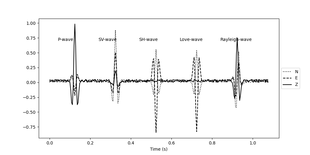
We start by generating a very simple synthetic data set for illustration purposes. The data will contain isolated wave arrivals for a P-wave, an SV-wave, an SH wave, a Love-wave, and a Rayleigh wave. To generate the data, we make use of the pure state polarization models that are implemented in the class ‘twistpy.polarization.PolarizationModel3C’.

# Generate an empty time series for each wave
N = 270  # Number of samples in the time series
signal1 = np.zeros((N, 3))  # Each signal has three components
signal2 = np.zeros((N, 3))
signal3 = np.zeros((N, 3))
signal4 = np.zeros((N, 3))
signal5 = np.zeros((N, 3))

dt = 1.0 / 250.0  # sampling interval
t = np.arange(0, signal1.shape[0]) * dt  # time axis
wavelet, t_wav, wcenter = ricker(
    t, 30.0
)  # generate a Ricker wavelet with 30 Hz center frequency
wavelet = wavelet[wcenter - int(len(t) / 2) : wcenter + int(len(t) / 2)]
wavelet_hilb = np.imag(
    hilbert(wavelet)
)  # Here we make use of the Hilbert transform to generate a Ricker wavelet
# with a 90 degree phase shift. This is to account for the fact that, for Rayleigh waves, the horizontal components are
# phase-shifted by 90 degrees with respect to the other components.

We now generate the relative amplitudes with which the waves are recorded on the three-component seismometer. All waves will arrive with a propagation azimuth of 30 degrees (ecxept for the P-wave, which we specify to have an azimuth of 60 degrees), the body waves will have an inclination angle of 20 degrees. The local P-wave and S-wave velocities at the recording station are assumed to be 1000 m/s and 400 m/s, respectively. The Rayleigh wave ellipticity angle is set to be -45 degrees resulting in a circular polarization.

wave1 = PolarizationModel3C(
    wave_type="P", theta=20.0, phi=60.0, vp=1000.0, vs=400.0, free_surface=True
)
# Generate a P-wave polarization model for
# a P-wave recorded at the free surface with an inclination of 20 degrees, an azimuth of 60 degrees. The local P- and
# S-wave velocities are 1000 m/s and 400 m/s
wave2 = PolarizationModel3C(
    wave_type="SV", theta=20.0, phi=30.0, vp=1000.0, vs=400.0, free_surface=True
)  # Generate an SV-wave polarization model
wave3 = PolarizationModel3C(wave_type="SH", theta=20.0, phi=30.0, free_surface=True)
# Generate an SH-wave polarization model
wave4 = PolarizationModel3C(
    wave_type="L", phi=30.0
)  # Generate a Love-wave polarization model
wave5 = PolarizationModel3C(
    wave_type="R", phi=30.0, xi=-45.0
)  # Generate a Rayleigh-wave polarization model with a
# Rayleigh wave ellipticity angle of -45 degrees.

Now we populate our signal with the computed amplitudes by setting a spike with the respective amplitude onto the different locations of the time axis. Then we convolve the data with the Ricker wavelet to generate our synthetic test seismograms.

signal1[30, :] = wave1.polarization.real.T
signal2[80, :] = wave2.polarization.real.T
signal3[130, :] = wave3.polarization.real.T
signal4[180, :] = wave4.polarization.real.T
signal5[230, 2:] = np.real(wave5.polarization[2:].T)
signal5[230, 0:2] = np.imag(wave5.polarization[0:2].T)

for j in range(0, signal1.shape[1]):
    signal1[:, j] = convolve(signal1[:, j], wavelet, mode="same")
    signal2[:, j] = convolve(signal2[:, j], wavelet, mode="same")
    signal3[:, j] = convolve(signal3[:, j], wavelet, mode="same")
    signal4[:, j] = convolve(signal4[:, j], wavelet, mode="same")
    if (
        j == 0 or j == 1
    ):  # Special case for horizontal translational components of the Rayleigh wave
        signal5[:, j] = convolve(signal5[:, j], wavelet_hilb, mode="same")
    else:
        signal5[:, j] = convolve(signal5[:, j], wavelet, mode="same")

signal = signal1 + signal2 + signal3 + signal4 + signal5  # sum all signals together
noise = rng.random((signal.shape))

signal += 0.05 * noise
# Plot the data
plt.figure(figsize=(10, 5))
plt.plot(t, signal[:, 0], "k:", label="N")
plt.plot(t, signal[:, 1], "k--", label="E")
plt.plot(t, signal[:, 2], "k", label="Z")
plt.text((30 - 20) * dt, 0.7, "P-wave")
plt.text((80 - 20) * dt, 0.7, "SV-wave")
plt.text((130 - 20) * dt, 0.7, "SH-wave")
plt.text((180 - 20) * dt, 0.7, "Love-wave")
plt.text((230 - 20) * dt, 0.7, "Rayleigh-wave")
plt.legend(loc="center left", bbox_to_anchor=(1, 0.5))
plt.xlabel("Time (s)")

Text(0.5, 25.722222222222214, 'Time (s)')

To make the synthetics accessible to TwistPy, we convert them to an Obspy Stream object.

data = Stream()
for n in range(signal.shape[1]):
    trace = Trace(
        data=signal[:, n],
        header={"delta": t[1] - t[0], "npts": int(signal.shape[0]), "starttime": 0.0},
    )
    data += trace

We now have our toy data ready that we want to use for polarization analysis and filtering. First, we need to specify the window parameters of the time-frequency window, within which the covariance matrices will be averaged. Here we specify a window that is frequency-dependent and extends over a single period in time (1/frequency). In the frequency-direction the window extends over 5 Hz.

window = {"number_of_periods": 1, "frequency_extent": 50.0}

Now we set up the polarization analysis. We use a value of k=1 for the S-transform.

analysis = TimeFrequencyAnalysis3C(
    N=data[0], E=data[1], Z=data[2], window=window, timeaxis="rel", k=1
)

Computing covariance matrices...
Covariance matrices computed!

To compute the polarization attributes, we run:

analysis.polarization_analysis()

Computing polarization attributes...
Polarization attributes have been computed!

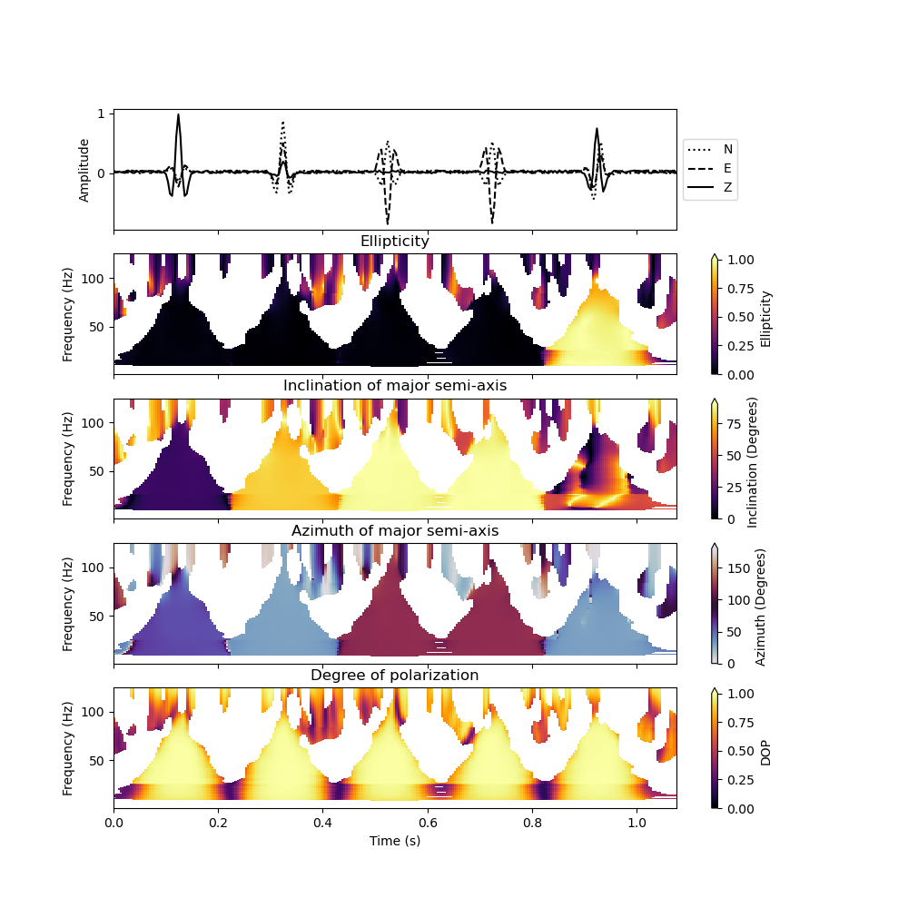
To plot the result, we can make use of the plot() method. We want to plot the inclination and azimuth of the major semi-axis of the polarization ellipse and only plot the polarization attributes at time frequency points where the signal strength in all three-components exceeds 5 percent of the maximum value:

analysis.plot(major_semi_axis=True, clip=0.05, show=False)

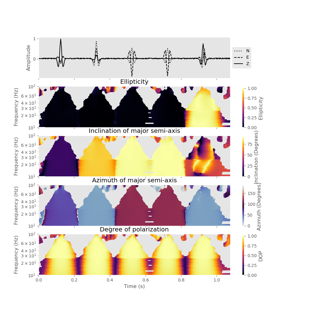
You can also plot the polarization attributes with a logarithmic frequency axis and restrict the frequency range that is plotted (here we only plot results between 10 Hz and 100 Hz).

analysis.plot(major_semi_axis=True, clip=0.05, show=False, log_frequency=True, fmin=10., fmax=100.)

We can now use the computed polarization attributes to devise a polarization filter. Depending on the number of samples in the seismograms, the computation of the polarization attributes can become quite expensive. If you do not want to recompute the polarization attributes, everytime you try a new filter, consider saving them to disk with:

analysis.save("my_analysis.pkl")

To reload your analysis from the disk, use:

analysis = load_analysis("my_analysis.pkl")

Once the polarization attributes are computed, you can access them as c lass attributes. The available attributes are: ‘dop’ (degree of polarization), ‘elli’ (Ellipticity), ‘inc1’ (Inclination of the major semi-axis of the polarization ellipse), ‘inc2’ (Inclination of the minor semi-axis), ‘azi1’ (Azimuth of the major semi-axis), and ‘azi2’ (Azimuth of the minor semi-axis). So, for example, if you want to access the ellipticity, you would do:

elli = analysis.elli

The corresponding frequency and time axes are:

time = analysis.t_pol
frequency = analysis.f_pol

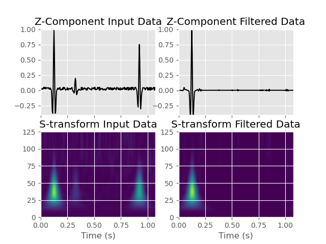
Now, let us devise a simple polarization filter. For this, we make use of the filter() method. The method takes arbitrary polarization attributes as an input for filtering. For example, we can devise a filter that will only keep the parts of the signal that are rectilinearly polarized (i.e., low ellipticity below 0.2), show a high degree of polarization (larger than 0.7), and that have a predominantly vertical polarization (inclination angle of the major semi-axis smaller than 40). The inclination is measured from the vertical axis downward, meaning that a wave at completely vertical incidence has an inclination of 0 degrees.

data_filtered = analysis.filter(
    plot_filtered_attributes=True, elli=[0.0, 0.2], dop=[0.7, 1], inc1=[0, 40]
)

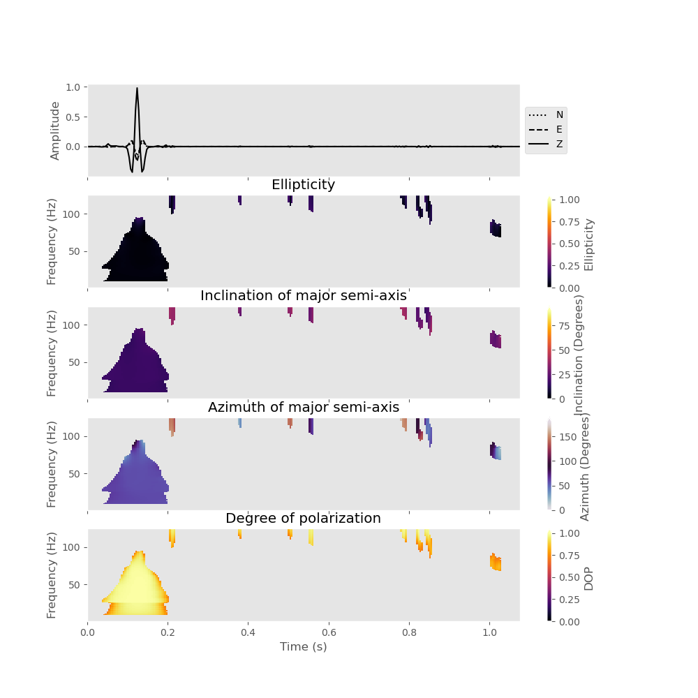
If we have a look at the output of this filter both in the time-domain and in the S-transform, we will see that only the P-wave is retained, while all other signals are suppressed.

# Compute S-transform of vertical component for plotting
Z_stran, f = stransform(data[2].data, k=1)
Z_stran_filtered, _ = stransform(
    data_filtered[0].data, k=1
)  # S-transform of filtered data for comparison
f /= dt

# Plot the result
fig, ax = plt.subplots(2, 2, sharex=True)
ax[0, 0].plot(analysis.t_pol, data[2].data, "k")
ax[0, 0].set_title("Z-Component Input Data")
ax[0, 0].set_ylim([-0.4, 1])
ax[1, 0].imshow(
    np.abs(Z_stran),
    origin="lower",
    aspect="auto",
    vmin=0,
    vmax=0.2,
    extent=[
        analysis.t_pol[0],
        analysis.t_pol[-1],
        analysis.f_pol[0],
        analysis.f_pol[-1],
    ],
)
ax[1, 0].set_xlabel("Time (s)")
ax[1, 0].set_title("S-transform Input Data")

ax[0, 1].plot(analysis.t_pol, data_filtered[0].data, "k")
ax[0, 1].set_title("Z-Component Filtered Data")
ax[0, 1].set_ylim([-0.4, 1])
ax[1, 1].imshow(
    np.abs(Z_stran_filtered),
    origin="lower",
    aspect="auto",
    vmin=0,
    vmax=0.2,
    extent=[
        analysis.t_pol[0],
        analysis.t_pol[-1],
        analysis.f_pol[0],
        analysis.f_pol[-1],
    ],
)
ax[1, 1].set_xlabel("Time (s)")
ax[1, 1].set_title("S-transform Filtered Data")

Text(0.5, 1.0, 'S-transform Filtered Data')

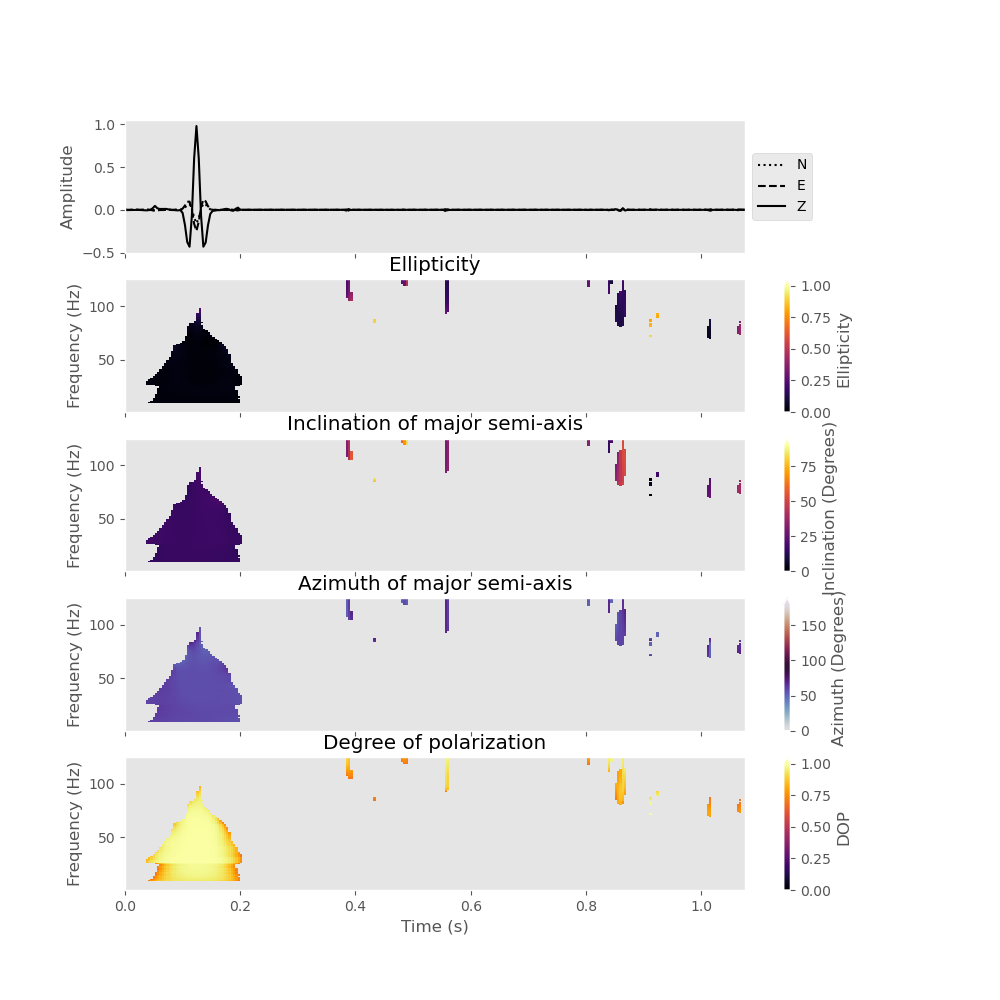
Similarly, we could devise a filter that only retains the elliptically polarized parts of the signal (e.g., surface waves).

data_filtered_rayleigh = analysis.filter(
    plot_filtered_attributes=True, elli=[0.7, 1.0], dop=[0.7, 1]
)

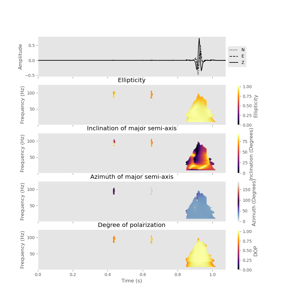
To filter out parts of the signal that exhibit particle motion along a specific direction (e.g., an azimuth around 60 degrees), we could use:

data_filtered_60degrees_azimuth = analysis.filter(
    plot_filtered_attributes=True, azi1=[50, 70], dop=[0.7, 1]
)

plt.show()