Note
Go to the end to download the full example code
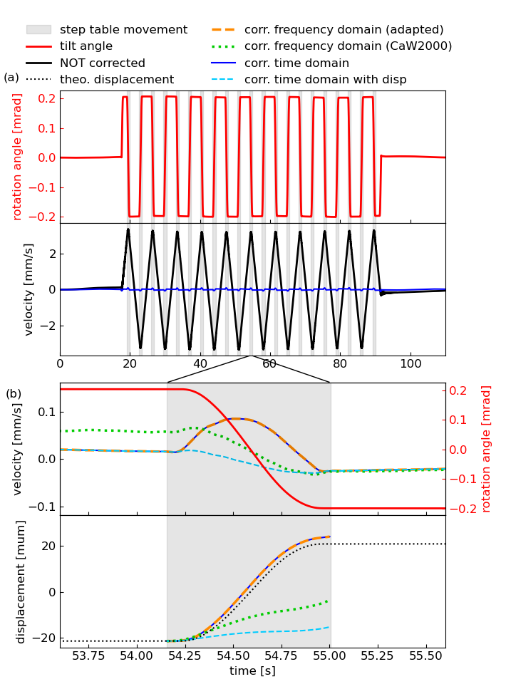
Tilt correction#
This script implements a simple example for dynamic tilt correction. It reproduces the tilt table experiment from Bernauer et al (2020) based on the method by Crawford and Webb (2000).
The example demonstrates the different correction variants provided by twistpy.tilt.correction.remove_tilt.
The example data required by this script is included in the TwistPy example_data collection.
import os

import numpy as np
from matplotlib import pyplot as plt
from matplotlib import rc
from matplotlib.transforms import Bbox, TransformedBbox, blended_transform_factory
from mpl_toolkits.axes_grid1.inset_locator import (
    BboxPatch,
    BboxConnector,
    BboxConnectorPatch,
)
from obspy import Stream, Trace

from twistpy.tilt.correction import remove_tilt
from twistpy.tilt.util import (
    get_data,
    trigger,
    calc_residual_disp,
    get_angle,
    theo_resid_disp,
    calc_height_of_mass,
)
This script implements a simple example for dynamic tilt correction. It reproduces the # tilt table experiment from Bernauer et al. 2020 (SRL).
data_dir = "../example_data/tilt_correction"
This method is needed for the matplotlib zoom effect
def connect_bbox(
    bbox1, bbox2, loc1a, loc2a, loc1b, loc2b, prop_lines, prop_patches=None
):
    if prop_patches is None:
        prop_patches = {
            **prop_lines,
            "alpha": prop_lines.get("alpha", 1) * 0.0,
        }

    c1 = BboxConnector(bbox1, bbox2, loc1=loc1a, loc2=loc2a, **prop_lines)
    c1.set_clip_on(False)
    c2 = BboxConnector(bbox1, bbox2, loc1=loc1b, loc2=loc2b, **prop_lines)
    c2.set_clip_on(False)

    bbox_patch1 = BboxPatch(bbox1, **prop_patches)
    bbox_patch2 = BboxPatch(bbox2, **prop_patches)

    p = BboxConnectorPatch(
        bbox1, bbox2, loc1a=loc1a, loc2a=loc2a, loc1b=loc1b, loc2b=loc2b, **prop_patches
    )
    p.set_clip_on(False)

    return c1, c2, bbox_patch1, bbox_patch2, p
This method is needed for the matplotlib zoom effect
def zoom_effect01(ax1, ax2, xmin, xmax, **kwargs):
    """
    Connect *ax1* and *ax2*. The *xmin*-to-*xmax* range in both axes will
    be marked.
    Parameters
    ----------
    ax1
        The main axes.
    ax2
        The zoomed axes.
    xmin, xmax
        The limits of the colored area in both plot axes.
    **kwargs
        Arguments passed to the patch constructor.
    """

    trans1 = blended_transform_factory(ax1.transData, ax1.transAxes)
    trans2 = blended_transform_factory(ax2.transData, ax2.transAxes)

    bbox = Bbox.from_extents(xmin, 0, xmax, 1)

    mybbox1 = TransformedBbox(bbox, trans1)
    mybbox2 = TransformedBbox(bbox, trans2)

    prop_patches = {**kwargs, "ec": "none", "alpha": 0.0}

    c1, c2, bbox_patch1, bbox_patch2, p = connect_bbox(
        mybbox1,
        mybbox2,
        loc1a=3,
        loc2a=2,
        loc1b=4,
        loc2b=1,
        prop_lines=kwargs,
        prop_patches=prop_patches,
    )

    ax1.add_patch(bbox_patch1)
    ax2.add_patch(bbox_patch2)
    ax2.add_patch(c1)
    ax2.add_patch(c2)
    ax2.add_patch(p)

    return c1, c2, bbox_patch1, bbox_patch2, p
This method is needed for the matplotlib zoom effect
def zoom_effect02(ax1, ax2, **kwargs):
    """
    ax1 : the main axes
    ax1 : the zoomed axes
    Similar to zoom_effect01.  The xmin & xmax will be taken from the
    ax1.viewLim.
    """

    tt = ax1.transScale + (ax1.transLimits + ax2.transAxes)
    trans = blended_transform_factory(ax2.transData, tt)

    mybbox1 = ax1.bbox
    mybbox2 = TransformedBbox(ax1.viewLim, trans)

    prop_patches = {**kwargs, "ec": "none", "alpha": 0.2}

    c1, c2, bbox_patch1, bbox_patch2, p = connect_bbox(
        mybbox1,
        mybbox2,
        loc1a=2,
        loc2a=3,
        loc1b=1,
        loc2b=4,
        prop_lines=kwargs,
        prop_patches=prop_patches,
    )

    ax1.add_patch(bbox_patch1)
    ax2.add_patch(bbox_patch2)
    ax2.add_patch(c1)
    ax2.add_patch(c2)
    ax2.add_patch(p)

    return c1, c2, bbox_patch1, bbox_patch2, p
- TEST - tilt table - #
high gain, 1/6 - #
166.7mum - #
21 steps - #
Get raw data from
stream1 = os.path.join(data_dir, "XX.TC120..HH*.D.2018.343")
stream2 = os.path.join(data_dir, "XX.BS1..HJ*.D.2018.343")
at the time
utctime = "2018-12-09T19:48:48.6"
how many seconds of data do you want to read in?
duration = 120
Define the seismometer and rotational sensor stream identifiers
correct_channel = "HH*"
input_channel = "HJ*"
Set some trigger parameters and start to search for steps from second
S = 18.0
# no steps after second
E = 91.0
correct the trigger onset by a constant offset, which was determined visually
c_on = -0.075
c_off = 0.49
define the zoom windows for the plots
zoom00 = 0.0
zoom01 = 110.0
zoom0 = 53.6
zoom1 = 55.6
Geometrical parameters of the experiment horizontal distance of center of seismometer to axis of rotation in m
l = 0.32  # noqa
# vertical distance of bottom of seismometer to axis of rotation in m
dh = 0.047
define the source stream (ss) and the receiver stream (sr) channels
ch_sr = "HHN"
ch_ss = "HJE"
get the data
vel_orig, rr_orig = get_data(
    stream1,
    stream2,
    utctime,
    duration,
    correct_channel,
    input_channel,
    os.path.join(data_dir, "station.xml"),
    ch_sr,
    ch_ss,
)
make four independent streams containing tilt contaminated acceleration recordings: (1) the original tilt contaminated stream for later comparisons (2) the stream that will be treated with the frequency domain (CaW) correction (3) the stream that will be treated with the frequency domain (coh) correction (4) the stream that will be treated with the time domain correction
sr = vel_orig.copy()
sr.filter("bandpass", freqmin=0.03, freqmax=10, corners=8, zerophase=True)

acc_orig = sr.copy()
acc_orig.differentiate()  # original acc recording (reciever)

rf1 = sr.copy()
rf2 = sr.copy()
rt = sr.copy()
rf1.differentiate()  # reciever for freq-domain (coh) analysis (acc recording)
rf2.differentiate()  # reciever for freq-domain (plain) analysis (acc recording)  # noqa
rt.differentiate()  # reciever for time-domain analysis (acc recording)
<obspy.core.stream.Stream object at 0x1813c90a0>
make two independent streams containing the tilt angle recording (1) original tilt angle recording for later comparisons (2) tilt angle recording as the source for the corrections
ss = rr_orig.copy()
ss.filter("bandpass", freqmin=0.03, freqmax=10, corners=8, zerophase=True)

ra_orig = ss.copy()
ra_orig.integrate()  # original rotation angle recording (source)

ts = ss.copy()
ts.integrate()  # source for correction (tilt angle recording)
<obspy.core.stream.Stream object at 0x181894b20>
In this example, we are treating the North-axis of acceleration and the East-axis of rotation angle. Thus, for a positive rotation, the tilt induced accelertion shows into the same direction as the horizontal ground movement accelertion. We account for this in the subsequent analysis by setting
par = True
Now, lets do the tilt corrections!
frequency domain (coh)#
fmin = None
fmax = None
acc_corr_freq1_data = remove_tilt(
    rf1[0].data,
    ts[0].data,
    rf1[0].stats.delta,
    fmin,
    fmax,
    parallel=par,
    smooth=100.0 / 164.0,
    method="coh",
)

acc_corr_freq1 = acc_orig.copy()
acc_corr_freq1[0].data = acc_corr_freq1_data

acc_corr_freq1.detrend("demean")

vel_corr_freq1 = acc_corr_freq1.copy()
vel_corr_freq1.integrate()

# -----------------------------------------------------------------------------
# frequency domain (plain)
# -----------------------------------------------------------------------------

fmin = None
fmax = None
acc_corr_freq2_data = remove_tilt(
    rf2[0].data,
    ts[0].data,
    rf2[0].stats.delta,
    fmin,
    fmax,
    parallel=par,
    smooth=100.0 / 164.0,
    method="freq",
)

acc_corr_freq2 = acc_orig.copy()
acc_corr_freq2[0].data = acc_corr_freq2_data

acc_corr_freq2.detrend("demean")

vel_corr_freq2 = acc_corr_freq2.copy()
vel_corr_freq2.integrate()

# -----------------------------------------------------------------------------
# time domain
# -----------------------------------------------------------------------------

acc_corr_time_data = remove_tilt(
    rt[0].data, ts[0].data, rt[0].stats.delta, parallel=par
)
acc_corr_time = acc_orig.copy()
acc_corr_time[0].data = acc_corr_time_data

acc_corr_time.detrend("demean")

vel_corr_time = acc_corr_time.copy()
vel_corr_time.integrate()
<obspy.core.stream.Stream object at 0x18204c580>
Due to the very well known geometry in the tilt table experiment, we can play some games e.g. try to locate the proof mass of the seismometer and compare the output of our corrections with theortically expercted movements.
on, off = trigger(rr_orig[0], 10, 140, 6.0, 5.0, c_on, c_off, S, E, plot=False)

# define a time axis
sec = np.arange(len(acc_orig[0].data)) / (acc_orig[0].stats.sampling_rate)

print(len(on))
print(len(off))

# calculate residual displacement

alpha = get_angle(ts, on, off)  # angle steps recorded by BS1
21
21
in theory: according to Steffen position of the mass is approximately at the middle of the housing
h_m = 0.0575  # m
h = h_m  # m

std_m = 0.01

r, centr = theo_resid_disp(ts[0].data, l, h, dh, rr_orig[0].data)
trr = Stream(traces=Trace(data=r, header=ts[0].stats))
trr.differentiate()
trr_a = trr.copy()
trr_a.differentiate()
time_ttheo, disp_ttheo, mean_disp_ttheo, sigma_ttheo = calc_residual_disp(
    trr, on, off, np.zeros(len(r)), theo=True
)
h_ttheo, std_ttheo = calc_height_of_mass(mean_disp_ttheo, l, dh, alpha)

tcentr = Stream(traces=Trace(data=centr, header=ts[0].stats))
tcentr.detrend("demean")
tcentr.detrend("linear")
tcentr.integrate()
tcentr.detrend("demean")
tcentr.detrend("linear")
tcentr.integrate()
<obspy.core.stream.Stream object at 0x1812e7ca0>
correct for residual displacement in time domain
acc_corr_time2 = acc_corr_time.copy()
acc_corr_time2[0].data = acc_corr_time2[0].data - trr_a[0].data

vel_corr_time2 = acc_corr_time2.copy()
vel_corr_time2.integrate()

tr1_vel = vel_corr_freq1.copy()
tr2_vel = vel_corr_freq2.copy()
tt_vel = vel_corr_time.copy()
tt2_vel = vel_corr_time2.copy()

tr1_new = vel_corr_freq1.copy()
tr2_new = vel_corr_freq2.copy()
tt_new = vel_corr_time.copy()
tt2_new = vel_corr_time2.copy()

time_tr1, disp_tr1, mean_disp_tr1, sigma_tr1 = calc_residual_disp(tr1_new, on, off, r)

time_tr2, disp_tr2, mean_disp_tr2, sigma_tr2 = calc_residual_disp(tr2_new, on, off, r)

time_tt, disp_tt, mean_disp_tt, sigma_tt = calc_residual_disp(tt_new, on, off, r)

time_tt2, disp_tt2, mean_disp_tt2, sigma_tt2 = calc_residual_disp(tt2_new, on, off, r)
calculate the position of the seismometer mass
h_tr1, std_tr1 = calc_height_of_mass(mean_disp_tr1, l, dh, alpha)
h_tr2, std_tr2 = calc_height_of_mass(mean_disp_tr2, l, dh, alpha)
h_tt, std_tt = calc_height_of_mass(mean_disp_tt, l, dh, alpha)

disp_corr_freq1 = vel_corr_freq1.copy()
disp_corr_freq1.integrate()

disp_corr_freq2 = vel_corr_freq2.copy()
disp_corr_freq2.integrate()

disp_corr_time = vel_corr_time.copy()
disp_corr_time.integrate()

disp_corr_time2 = vel_corr_time2.copy()
disp_corr_time2.integrate()

# -----------------------------------------------------------------------------
# OUTPUT
# -----------------------------------------------------------------------------
scale = 1.0e3
scaled = 1.0e6

print("-----------------------------------------------")
print("mean residual displacement:")
print(
    "frequency domain (coh): %.3f +/- %.3f mm"
    % (mean_disp_tr1 * scale, sigma_tr1 * scale)
)
print(
    "frequency domain (CaW): %.3f +/- %.3f mm"
    % (mean_disp_tr2 * scale, sigma_tr2 * scale)
)
print(
    "time domain           : %.3f +/- %.3f mm"
    % (mean_disp_tt * scale, sigma_tt * scale)
)
print("")
print("-----------------------------------------------")
print("height of seismometer mass:")
print("frequency domain (coh): %.3f +/- %.3f mm" % (h_tr1 * scale, std_tr1 * scale))
print("frequency domain (CaW): %.3f +/- %.3f mm" % (h_tr2 * scale, std_tr2 * scale))
print("time domain           : %.3f +/- %.3f mm" % (h_tt * scale, std_tt * scale))
print("theoretical           : %.3f +/- %.3f mm" % (h_ttheo * scale, std_ttheo * scale))
print("measured              : %.3f +/- %.3f mm" % (h_m * scale, std_m * scale))
print("-----------------------------------------------")
print("")
-----------------------------------------------
mean residual displacement:
frequency domain (coh): 0.042 +/- 0.005 mm
frequency domain (CaW): 0.016 +/- 0.002 mm
time domain           : 0.042 +/- 0.005 mm

-----------------------------------------------
height of seismometer mass:
frequency domain (coh): 57.400 +/- 0.235 mm
frequency domain (CaW): -6.458 +/- 0.091 mm
time domain           : 57.400 +/- 0.235 mm
theoretical           : 57.161 +/- 0.234 mm
measured              : 57.500 +/- 10.000 mm
-----------------------------------------------
Plots#
Uncomment the following lines in case you want to use latex for type setting
# params = {
#     'text.usetex': True,
#     'text.latex.preamble': [
#         r'\usepackage{cmbright}', r'\usepackage{amsmath}']}
# plt.rcParams.update(params)
plt.rcParams["figure.figsize"] = 7.1, 9.6
sizeOfFont = 12
fontProperties = {"weight": "normal", "size": sizeOfFont}
rc("font", **fontProperties)

# -----------------------------------------------------------------------------
# colors and linestyles
# define colors
al_trig = 0.1

c_trig_on = (0, 0, 0)
c_trig_off = (0, 0, 0)

c_angle = (1, 0, 0)
c_vel = (0, 0, 0)

c_time = (0, 0, 1)
c_time2 = (0, 0.8, 1)
c_coh = (1, 0.54, 0)
c_freq = (0, 0.8, 0)

c_tdisp = (0, 0, 0)

# define linestyles
ls_trig_on = "-"
ls_trig_off = "-"

ls_angle = "-"
ls_vel = "-"

ls_time = "-"
ls_time2 = "--"
ls_coh = "--"
ls_freq = ":"

ls_tdisp = ":"

# define linewidth
lw_trig_on = 2.0
lw_trig_off = 2.0

lw_angle = 2.0
lw_vel = 2.0

lw_time = 1.5
lw_time2 = 1.5
lw_coh = 2.5
lw_freq = 2.5

lw_tdisp = 2.0

# define labels
l_trig = "step table movement"

l_angle = "tilt angle"
l_vel = "NOT corrected"

l_time = "corr. time domain"
l_time2 = "corr. time domain with disp"
l_coh = "corr. frequency domain (adapted)"
l_freq = "corr. frequency domain (CaW2000)"

l_tdisp = "theo. displacement"
# END colors and linestyles
gridspec = dict(hspace=0.0, height_ratios=[1, 1, 0.2, 1, 1])
fig, axs = plt.subplots(nrows=5, ncols=1, gridspec_kw=gridspec)
axs[2].set_visible(False)

ax0 = axs[0]
ax2 = axs[1]
ax3 = axs[3]
ax31 = ax3.twinx()
ax4 = axs[4]

(line_angle,) = ax0.plot(
    sec,
    ts[0].data * scale,
    color=c_angle,
    linestyle=ls_angle,
    linewidth=lw_angle,
    label=l_angle,
)

for i in range(len(on)):
    p_trig = ax0.axvspan(on[i], off[i], alpha=al_trig, color=c_trig_on)

(line_vel,) = ax2.plot(
    sec,
    vel_orig[0].data * scale,
    color=c_vel,
    linestyle=ls_vel,
    linewidth=lw_vel,
    label=l_vel,
)

(line_time,) = ax2.plot(
    sec,
    tt_vel[0].data * scale,
    color=c_time,
    linestyle=ls_time,
    linewidth=lw_time,
    label=l_time,
)

for i in range(len(on)):
    ax2.axvspan(on[i], off[i], alpha=al_trig, color=c_trig_on)

(line_angle,) = ax31.plot(
    sec,
    ts[0].data * scale,
    color=c_angle,
    linestyle=ls_angle,
    linewidth=lw_angle,
    label=l_angle,
)

for i in range(len(on)):
    p_trig = ax31.axvspan(on[i], off[i], alpha=al_trig, color=c_trig_on)

(line_time,) = ax3.plot(
    sec,
    tt_vel[0].data * scale,
    color=c_time,
    linestyle=ls_time,
    linewidth=lw_time,
    label=l_time,
)

(line_coh,) = ax3.plot(
    sec,
    tr1_vel[0].data * scale,
    color=c_coh,
    linestyle=ls_coh,
    linewidth=lw_coh,
    label=l_coh,
)

(line_freq,) = ax3.plot(
    sec,
    tr2_vel[0].data * scale,
    color=c_freq,
    linestyle=ls_freq,
    linewidth=lw_freq,
    label=l_freq,
)

(line_time2,) = ax3.plot(
    sec,
    vel_corr_time2[0].data * scale,
    color=c_time2,
    linestyle=ls_time2,
    linewidth=lw_time2,
    label=l_time2,
)

for i in range(len(on)):
    ax4.axvspan(on[i], off[i], alpha=al_trig, color=c_trig_on)

    (line_time_d,) = ax4.plot(
        time_tt[i],
        disp_tt[i] * scaled,
        color=c_time,
        linestyle=ls_time,
        linewidth=lw_time,
        label=l_time,
    )

    (line_coh_d,) = ax4.plot(
        time_tr1[i],
        disp_tr1[i] * scaled,
        color=c_coh,
        linestyle=ls_coh,
        linewidth=lw_coh,
        label=l_coh,
    )

    (line_freq_d,) = ax4.plot(
        time_tr2[i],
        disp_tr2[i] * scaled,
        color=c_freq,
        linestyle=ls_freq,
        linewidth=lw_freq,
        label=l_freq,
    )

    (line_time_d2,) = ax4.plot(
        time_tt2[i],
        disp_tt2[i] * scaled,
        color=c_time2,
        linestyle=ls_time2,
        linewidth=lw_time2,
        label=l_time2,
    )

(line_theo_d,) = ax4.plot(
    sec, r * scaled, color=c_tdisp, linestyle=ls_tdisp, label=l_tdisp
)

ax0.set_ylabel("rotation angle [mrad]", color=c_angle)

ax2.set_ylabel("velocity [mm/s]")

ax3.set_ylabel("velocity [mm/s]")
ax31.set_ylabel("rotation angle [mrad]", color=c_angle)

ax4.set_ylabel("displacement [mum]")
ax4.set_xlabel("time [s]")

ax0.tick_params("y", colors=c_angle)
ax31.tick_params("y", colors=c_angle)

ax0.tick_params(direction="in")
ax2.tick_params(direction="in")
ax3.tick_params(direction="in")
ax31.tick_params(direction="in")
ax4.tick_params(direction="in")

ax0.set_xticklabels([])
ax31.set_xticklabels([])
ax3.set_xticklabels([])

ax0.text(-16, 0.26, "(a)")
ax3.text(53.32, 0.13, "(b)")

# legend
ba = (-0.098, 3.2)
lines = (
    p_trig,
    line_angle,
    line_vel,
    line_theo_d,
    line_coh,
    line_freq,
    line_time,
    line_time2,
)
labels = (l_trig, l_angle, l_vel, l_tdisp, l_coh, l_freq, l_time, l_time2)
plt.legend(
    lines, labels, loc=ba, bbox_transform=None, borderaxespad=0.0, frameon=False, ncol=2
)

ax0.set_xlim(zoom00, zoom01)
ax2.set_xlim(zoom00, zoom01)
ax3.set_xlim(zoom0, zoom1)
ax31.set_xlim(zoom0, zoom1)
ax4.set_xlim(zoom0, zoom1)

plt.subplots_adjust(top=0.868, bottom=0.053, left=0.118, right=0.88)

zoom_effect01(ax2, ax3, 54.16, 55.00)

plt.gcf().savefig("tilt_correction_step_table.png")

plt.show()
Total running time of the script: ( 0 minutes 1.826 seconds)