Six-component dispersion analysis

In this tutorial, you will learn how to extract dispersion curves and frequency-dependent Rayleigh wave ellipticity angles from single-station six-component recordings of ambient noise.

import numpy as np
from obspy.core import read

from twistpy.polarization import DispersionAnalysis
from twistpy.polarization.machinelearning import SupportVectorMachine

We start by reading in the data. The data corresponds to a recording of 2h40min of ambient noise recorded in the city of Munich with a BlueSeis rotational seismometer and a co-located seismometer. Both sensors were mounted on the same concrete base plate. With TwistPy, dispersion curves are estimated by 6C polarization analysis. First, Rayleigh waves and Love waves are detected using a machine learning algorithm. In time windows, where a Love or Rayleigh wave is detected, the phase velocity and ellipticity is estimated from the first eigenvector of the data covariance matrix. For polarization analysis, we convert our data to dimensionless units by scaling the translational components with a scaling velocity (see other examples on 6C polarization analysis). After scaling, the translational and rotational components should have comparable amplitudes. This makes the analysis more stable.

data = read("../example_data/6C_urban_noise.mseed")
scaling_velocity = 800.0
for i, trace in enumerate(data):
    if i < 3:
        trace.differentiate()
        trace.data /= scaling_velocity
    else:
        trace.data -= np.median(
            trace.data
        )  # Ensure that the rotational components have a median of 0
    trace.taper(0.05)

Now we train the machine learning model for the detection of Love and Rayleigh waves. We additionally train the model to be able to detect body waves because we want to avoid leakage of body waves into our Love and Rayleigh wave dispersion curves. We choose a velocity range that is typical for the near-surface in the frequency range we are interested in.

svm = SupportVectorMachine(name="dispersion_analysis2")
svm.train(
    wave_types=["R", "L", "P", "SV", "Noise"],
    scaling_velocity=scaling_velocity,
    phi=(0, 360),
    vp=(400, 3000),
    vp_to_vs=(1.7, 2.4),
    vr=(100, 3000),
    vl=(100, 3000),
    xi=(-90, 90),
    theta=(0, 80),
    C=100,
    plot_confusion_matrix=False,
)

A trained model already exists with this name and is saved at '/Users/Dave/Documents/TwistPyDocBuilding/TwistPy/twistpy/SVC_models/dispersion_analysis2.pkl'
Nothing will be done! Please delete the file above if you want to re-train this model.

We now have everything we need to extract dispersion curves from our ambient noise data. We specify that the time window for the analysis should stretch over 2 dominant periods at each frequency of interest. Additionally, we specify that neighbouring windows should overlap by half the window width in this case (‘overlap’: 0.5). We want to extract Love and Rayleigh wave dispersion curves in the frequency range between 1 and 20 Hz. The data is automatically filtered to various frequency bands in the interval 1 to 20 Hz, each frequency band extends over the number of octaves specified by the parameter ‘octaves’. Here, we choose quarter octave frequency bands.

window = {"number_of_periods": 3, "overlap": 0.5}
da = DispersionAnalysis(
    traN=data[1],
    traE=data[0],
    traZ=data[2],
    rotN=data[4],
    rotE=data[5],
    rotZ=data[3],
    window=window,
    scaling_velocity=scaling_velocity,
    verbose=True,
    fmin=1.0,
    fmax=20.0,
    octaves=0.25,
    svm=svm,
)

Estimating surface wave parameters at frequency f =  20.00 Hz. Frequency step 1 out of 18.
Estimating surface wave parameters at frequency f =  16.82 Hz. Frequency step 2 out of 18.
Estimating surface wave parameters at frequency f =  14.14 Hz. Frequency step 3 out of 18.
Estimating surface wave parameters at frequency f =  11.89 Hz. Frequency step 4 out of 18.
Estimating surface wave parameters at frequency f =  10.00 Hz. Frequency step 5 out of 18.
Estimating surface wave parameters at frequency f =  8.41 Hz. Frequency step 6 out of 18.
Estimating surface wave parameters at frequency f =  7.07 Hz. Frequency step 7 out of 18.
Estimating surface wave parameters at frequency f =  5.95 Hz. Frequency step 8 out of 18.
Estimating surface wave parameters at frequency f =  5.00 Hz. Frequency step 9 out of 18.
Estimating surface wave parameters at frequency f =  4.20 Hz. Frequency step 10 out of 18.
Estimating surface wave parameters at frequency f =  3.54 Hz. Frequency step 11 out of 18.
Estimating surface wave parameters at frequency f =  2.97 Hz. Frequency step 12 out of 18.
Estimating surface wave parameters at frequency f =  2.50 Hz. Frequency step 13 out of 18.
Estimating surface wave parameters at frequency f =  2.10 Hz. Frequency step 14 out of 18.
Estimating surface wave parameters at frequency f =  1.77 Hz. Frequency step 15 out of 18.
Estimating surface wave parameters at frequency f =  1.49 Hz. Frequency step 16 out of 18.
Estimating surface wave parameters at frequency f =  1.25 Hz. Frequency step 17 out of 18.
Estimating surface wave parameters at frequency f =  1.05 Hz. Frequency step 18 out of 18.

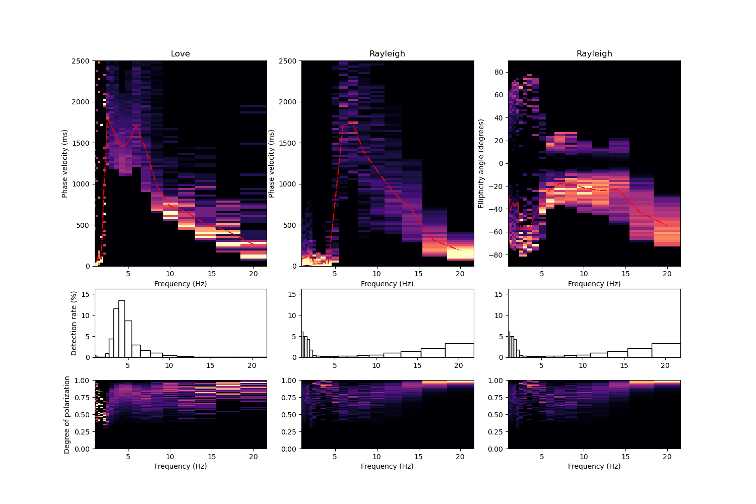
After running the analysis, we can save it to disk (e.g. da.save(‘dispersion_analysis.pkl’)) or simply plot it using the provided plot() method.

da.plot()

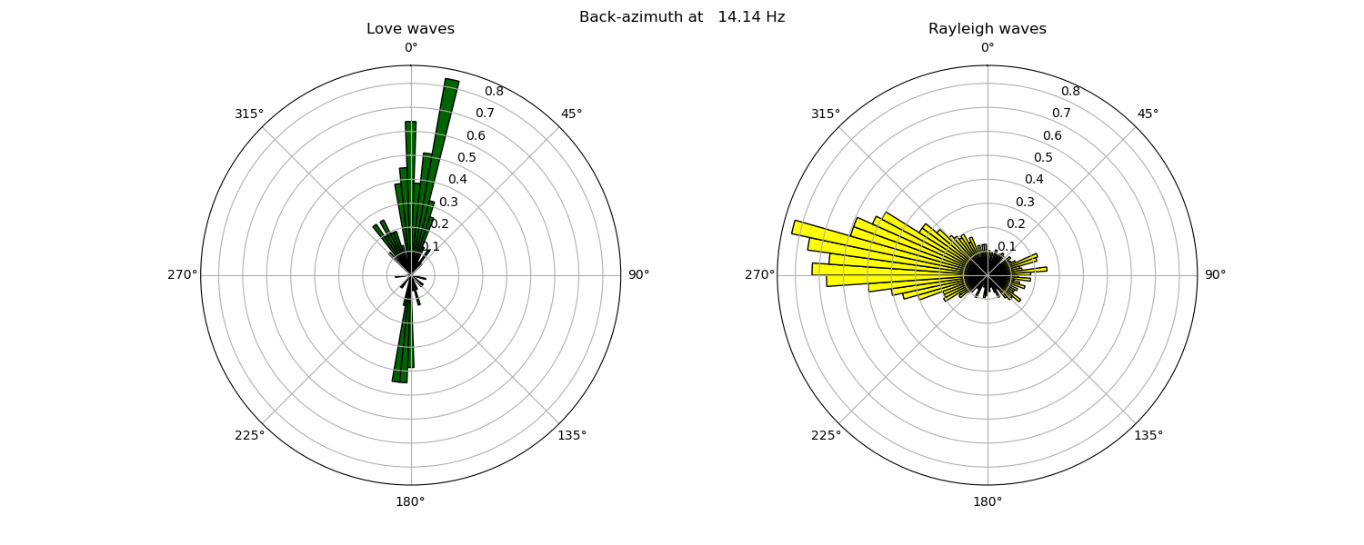
To plot the back-azimuth at a specific frequency, use the plot_baz() method:

da.plot_baz(freq=14.0)