Array Processing: Beamforming

In this tutorial, you will learn how to use TwistPy’s Array processing tools for beamforming.

import matplotlib.pyplot as plt
import numpy as np
from obspy.core import UTCDateTime

from twistpy.array_processing import BeamformingArray, plot_beam
from twistpy.convenience import generate_synthetics, to_obspy_stream

rng = np.random.default_rng(1)

# sphinx_gallery_thumbnail_number = 4

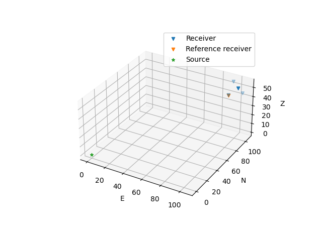
Instantiate an object of class BeamformingArray(), the basic interface that we use to perform array processing. We pass a name to uniquely identify the array and the coordinates of the receivers. The coordinates should be defined in a left-handed coordinate system as North, East, Up. Additionally, we specify the index of a reference receiver, all phase delays inside the array are computed with respect to this receiver:

# Define tetrahedral array coordinates
aperture = 5.0  # Array aperture in meters
center_point = np.asarray(
    [100, 100, 50]
)  # Coordinates of the center point of the array (meters)
# Array coordinates as (Nx3) array, with N being the number of receivers
coordinates = np.tile(center_point, (4, 1)) + aperture * np.array(
    [[-1, 1, 1], [1, -1, 1], [1, 1, -1], [-1, -1, -1]]
)

# Instantiate BeamformingArray object (the fourth receiver (with index 3) is specified to be the reference receiver)
array = BeamformingArray(name="My Array", coordinates=coordinates, reference_receiver=3)

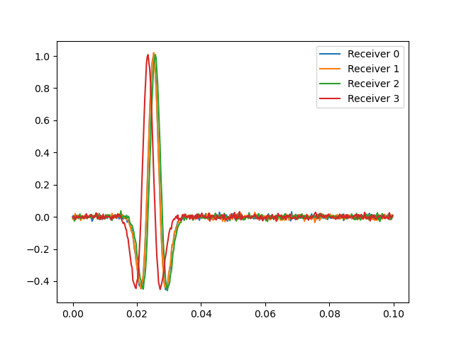
In this example, we generate some synthetic data with a source located at the origin:

source_coordinates = np.asarray([0, 0, 0])  # Source at the origin

Plot the source-receiver configuration:

fig = plt.figure()
ax = fig.add_subplot(projection="3d")
ax.scatter(
    array.coordinates[:, 1],
    array.coordinates[:, 0],
    array.coordinates[:, 2],
    marker="v",
)
ax.scatter(
    array.coordinates[array.reference_receiver, 1],
    array.coordinates[array.reference_receiver, 0],
    array.coordinates[array.reference_receiver, 2],
    marker="v",
)
ax.scatter(
    source_coordinates[1], source_coordinates[0], source_coordinates[2], marker="*"
)
ax.legend(["Receiver", "Reference receiver", "Source"])
ax.set_xlabel("E")
ax.set_ylabel("N")
ax.set_zlabel("Z")
ax.set_box_aspect((np.ptp(ax.get_xlim()), np.ptp(ax.get_ylim()), np.ptp(ax.get_zlim())))

Specify medium and data parameters for the computation of synthetics:

velocity = 6000  # Set medium velocity to 6000 m/s
dt = 2.5e-4  # sampling rate of seismograms (s)
tmax = 0.1  # total simulation time (s)
wavelet_center_frequency = 100  # wavelet center frequency in Hz
t = np.arange(0, tmax, dt)
nt = int(len(t))  # Number of samples

# Generate synthetic data using a Ricker wavelet
data = generate_synthetics(
    source_coordinates,
    array,
    t,
    velocity=velocity,
    center_frequency=wavelet_center_frequency,
)  # Use helper function to generate synthetics
data += rng.normal(scale=1e-2, size=data.shape)  # Add noise for numerical stability

# Plot data
plt.figure()
plt.plot(t, data.T)
plt.legend(["Receiver 0", "Receiver 1", "Receiver 2", "Receiver 3"])

<matplotlib.legend.Legend object at 0x188e256a0>

We now need to feed the data to our BeamformingArray object. BeamformingArray objects only accept data in ObsPy Stream() format. We therefore convert the synthetic data to an ObsPy Stream:

# Convert data to Obspy Stream format
start_time = UTCDateTime(2022, 2, 1, 10, 00, 00, 0)  # Recording time of first sample
data_st = to_obspy_stream(
    data, start_time, dt
)  # Use helper function to convert data to ObsPy Stream()
print(data_st)

# Add data to array object
array.add_data(
    data_st
)  # add_data() will automatically check that the data is in  Stream() format and that the
# number of traces in the data agrees with the number of receivers

4 Trace(s) in Stream:
XX.X00..XXX | 2022-02-01T10:00:00.000000Z - 2022-02-01T10:00:00.099750Z | 4000.0 Hz, 400 samples
XX.X01..XXX | 2022-02-01T10:00:00.000000Z - 2022-02-01T10:00:00.099750Z | 4000.0 Hz, 400 samples
XX.X02..XXX | 2022-02-01T10:00:00.000000Z - 2022-02-01T10:00:00.099750Z | 4000.0 Hz, 400 samples
XX.X03..XXX | 2022-02-01T10:00:00.000000Z - 2022-02-01T10:00:00.099750Z | 4000.0 Hz, 400 samples
Data successfully added to the BeamformingArray object!

Specify parameters for array processing: Frequency band over which to perform frequency-domain beamforming

freq_band = (90.0, 110.0)
inclination = (
    0,
    90,
    1,
)  # Search space for the inclination in degrees (min_value, max_value, increment)
azimuth = (
    0,
    360,
    1,
)  # Search space for the back-azimuth in degrees (min_value, max_value, increment)
velocity = 6000.0  # Intra-array velocity in m/s, either a float or a tuple as for azimuth and inclination if velocity
# is unknown and part of the search
number_of_sources = 1  # Specify the number of interfering sources that will be estimated in the time window
# (only relevant for MUSIC)

Now we have everything we need to compute the steering vectors:

array.compute_steering_vectors(
    frequency=np.mean(freq_band),
    inclination=inclination,
    azimuth=azimuth,
    intra_array_velocity=velocity,
)

Steering vectors computed!

Let’s now perform beamforming at a specific time. Currently, three different beamforming methods are implemented: ‘MUSIC’, ‘MVDR’ (minimum variance distortionless response or Capon Beamformer), and ‘BARTLETT’ (conventional beamforming). To compute the beam power at time=event_time, we do:

event_time = (
    start_time + 0.012
)  # Pick time, where the start of the analysis window is placed
# For a time dependent analysis, slide event_time down the trace
P_MUSIC = array.beamforming(
    method="MUSIC",
    event_time=event_time,
    frequency_band=freq_band,
    window=5,
    number_of_sources=number_of_sources,
)
P_MVDR = array.beamforming(
    method="MVDR", event_time=event_time, frequency_band=freq_band, window=5
)
P_BARTLETT = array.beamforming(
    method="BARTLETT", event_time=event_time, frequency_band=freq_band, window=5
)
# Window specifies the width of the time window, here corresponding to 5 times the dominant period in the specified
# frequency band
# If you want to perform a time-depenent analysis you would slide the window down the data by adjusting event_time

Plot the results. The azimuth is defined clock-wise from the North axis. The inclination is measured from the vertical axis downward. The extracted azimuth and inclination point into the direction of propagation of the wave (away from the source).

# Compute the true propagation direction at the center point of the array as a reference to evaluate beamforming
# performance
propagation_direction = center_point - source_coordinates
print(np.linalg.norm(propagation_direction))
propagation_direction = propagation_direction / np.linalg.norm(propagation_direction)

# negative to go from counter-clockwise to clockwise definition of angles
azimuth_true = np.arctan2(propagation_direction[1], propagation_direction[0])
if azimuth_true < 0:
    azimuth_true += 2 * np.pi
inclination_true = np.arctan(
    np.linalg.norm(propagation_direction[:-1]) / propagation_direction[2]
)

# Plot beamforming results obtained with the 3 different methods
fig_bf, ax_bf = plt.subplots(3, 1, sharex=True, sharey=True, figsize=(10, 12))
ax_bf[0].imshow(
    P_MUSIC,
    extent=[azimuth[0], azimuth[1], inclination[0], inclination[1]],
    origin="lower",
)
ax_bf[0].plot(np.degrees(azimuth_true), np.degrees(inclination_true), "r*")
ax_bf[0].set_xlabel("Azimuth (degrees)")
ax_bf[0].set_ylabel("Inclination (degrees)")
ax_bf[0].legend(["True"], loc="center left", bbox_to_anchor=(1, 0.5))
ax_bf[0].set_title("MUSIC")

ax_bf[1].imshow(
    P_MVDR,
    extent=[azimuth[0], azimuth[1], inclination[0], inclination[1]],
    origin="lower",
)
ax_bf[1].plot(np.degrees(azimuth_true), np.degrees(inclination_true), "r*")
ax_bf[1].set_xlabel("Azimuth (degrees)")
ax_bf[1].set_ylabel("Inclination (degrees)")
ax_bf[1].legend(["True"], loc="center left", bbox_to_anchor=(1, 0.5))
ax_bf[1].set_title("MVDR (Capon)")

ax_bf[2].imshow(
    P_BARTLETT,
    extent=[azimuth[0], azimuth[1], inclination[0], inclination[1]],
    origin="lower",
)
ax_bf[2].plot(np.degrees(azimuth_true), np.degrees(inclination_true), "r*")
ax_bf[2].set_xlabel("Azimuth (degrees)")
ax_bf[2].set_ylabel("Inclination (degrees)")
ax_bf[2].legend(["True"], loc="center left", bbox_to_anchor=(1, 0.5))
ax_bf[2].set_title("BARTLETT")

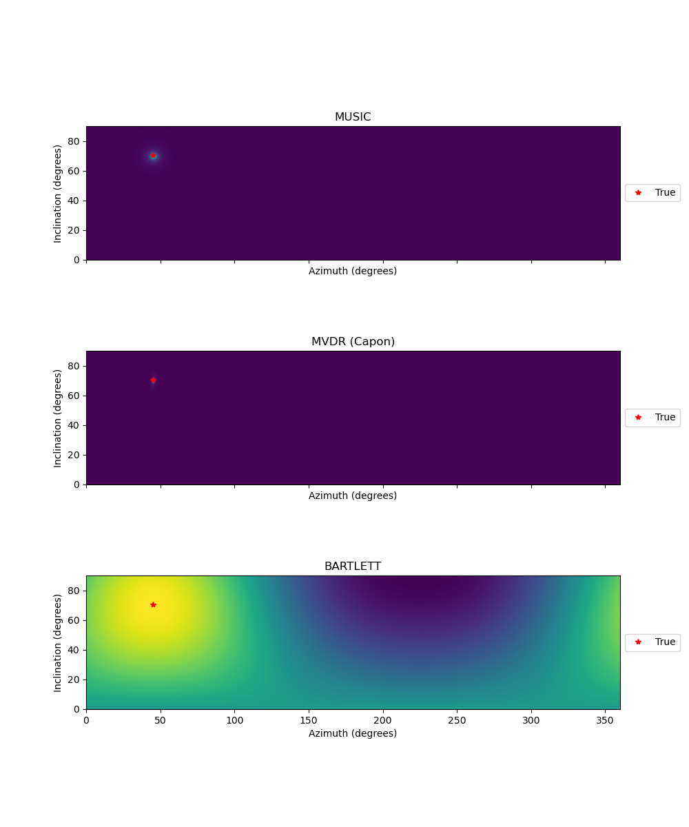
150.0

Text(0.5, 1.0, 'BARTLETT')

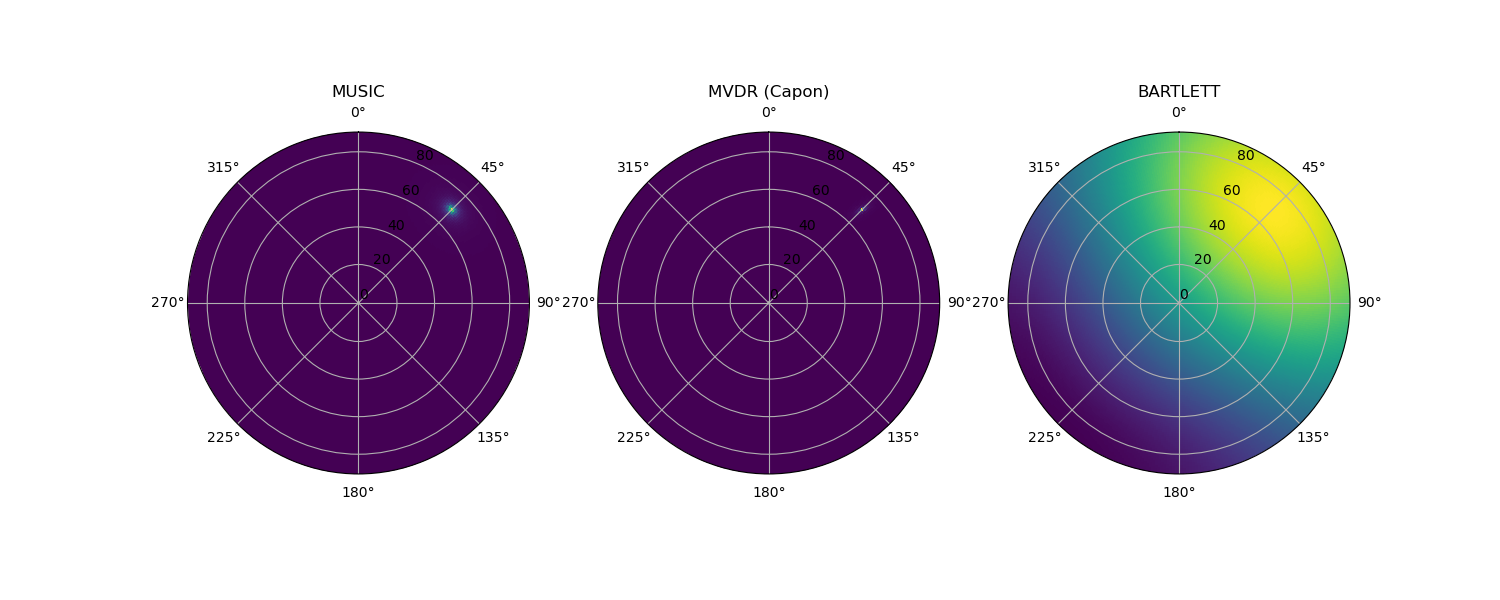
For a polar plot with the azimuth plotted as the polar angle and the inclination as the radius:

azi_plot = np.arange(azimuth[0], azimuth[1] + azimuth[2], azimuth[2])
inc_plot = np.arange(inclination[0], inclination[1] + inclination[2], inclination[2])

azi_plot, inc_plot = np.meshgrid(np.radians(azi_plot), inc_plot)

fig_bf_polar, ax_bf_polar = plt.subplots(
    1, 3, sharex=True, sharey=True, figsize=(15, 6), subplot_kw=dict(polar=True)
)
for ax_p in ax_bf_polar:
    ax_p.set_theta_direction(-1)
    ax_p.set_theta_offset(np.pi / 2.0)
ax_bf_polar[0].pcolormesh(azi_plot, inc_plot, P_MUSIC.squeeze())
ax_bf_polar[0].set_title("MUSIC")

ax_bf_polar[1].pcolormesh(azi_plot, inc_plot, P_MVDR.squeeze())
ax_bf_polar[1].set_title("MVDR (Capon)")

ax_bf_polar[2].pcolormesh(azi_plot, inc_plot, P_BARTLETT.squeeze())
ax_bf_polar[2].set_title("BARTLETT")

Text(0.5, 1.0773428912783753, 'BARTLETT')

To visualize the beam power in 3D, we use a simple back-projection of the beam assuming straight rays:

# Plot the beam in 3D domain
nx, ny, nz = (
    111,
    111,
    61,
)  # number of points in x-, y- and z- direction where beam is plotted
xmin, xmax = 0, 110  # min and max locations in x-direction where beam will be plotted
ymin, ymax = 0, 110
zmin, zmax = 0, 60
x = np.linspace(xmin, xmax, nx)
y = np.linspace(ymin, ymax, ny)
z = np.linspace(zmin, zmax, nx)

(
    X,
    Y,
    Z,
) = np.meshgrid(x, y, z)
grid = np.asarray([X.flatten(), Y.flatten(), Z.flatten()]).T
beam_origin = center_point  # location where the origin of the beam is located

# Plot the beam intensity for the four different methods
fig_beam, ax_beam = plt.subplots(
    3, 1, figsize=(10, 15), subplot_kw={"projection": "3d"}
)

plot_beam(
    grid, beam_origin, P_MUSIC, inclination, azimuth, ax=ax_beam[0]
)  # Helper function to plot the beam power
ax_beam[0].scatter(
    array.coordinates[:, 1],
    array.coordinates[:, 0],
    array.coordinates[:, 2],
    marker="v",
)
ax_beam[0].scatter(
    array.coordinates[array.reference_receiver, 1],
    array.coordinates[array.reference_receiver, 0],
    array.coordinates[array.reference_receiver, 2],
    marker="v",
)
ax_beam[0].scatter(
    source_coordinates[1], source_coordinates[0], source_coordinates[2], marker="*"
)
ax_beam[0].set_xlabel("E")
ax_beam[0].set_ylabel("N")
ax_beam[0].set_zlabel("Z")
ax_beam[0].set_box_aspect(
    (np.ptp(ax.get_xlim()), np.ptp(ax.get_ylim()), np.ptp(ax.get_zlim()))
)
ax_beam[0].set_title("MUSIC")

plot_beam(grid, beam_origin, P_MVDR, inclination, azimuth, ax=ax_beam[1], clip=0.05)
ax_beam[1].scatter(
    array.coordinates[:, 1],
    array.coordinates[:, 0],
    array.coordinates[:, 2],
    marker="v",
)
ax_beam[1].scatter(
    array.coordinates[array.reference_receiver, 1],
    array.coordinates[array.reference_receiver, 0],
    array.coordinates[array.reference_receiver, 2],
    marker="v",
)
ax_beam[1].scatter(
    source_coordinates[1], source_coordinates[0], source_coordinates[2], marker="*"
)
ax_beam[1].set_xlabel("E")
ax_beam[1].set_ylabel("N")
ax_beam[1].set_zlabel("Z")
ax_beam[1].set_box_aspect(
    (np.ptp(ax.get_xlim()), np.ptp(ax.get_ylim()), np.ptp(ax.get_zlim()))
)
ax_beam[1].set_title("MVDR (Capon)")

plot_beam(grid, beam_origin, P_BARTLETT, inclination, azimuth, ax=ax_beam[2], clip=0.8)
ax_beam[2].scatter(
    array.coordinates[:, 1],
    array.coordinates[:, 0],
    array.coordinates[:, 2],
    marker="v",
)
ax_beam[2].scatter(
    array.coordinates[array.reference_receiver, 1],
    array.coordinates[array.reference_receiver, 0],
    array.coordinates[array.reference_receiver, 2],
    marker="v",
)
ax_beam[2].scatter(
    source_coordinates[1], source_coordinates[0], source_coordinates[2], marker="*"
)
ax_beam[2].set_xlabel("E")
ax_beam[2].set_ylabel("N")
ax_beam[2].set_zlabel("Z")
ax_beam[2].set_box_aspect(
    (np.ptp(ax.get_xlim()), np.ptp(ax.get_ylim()), np.ptp(ax.get_zlim()))
)
ax_beam[2].set_title("BARTLETT")
plt.show()

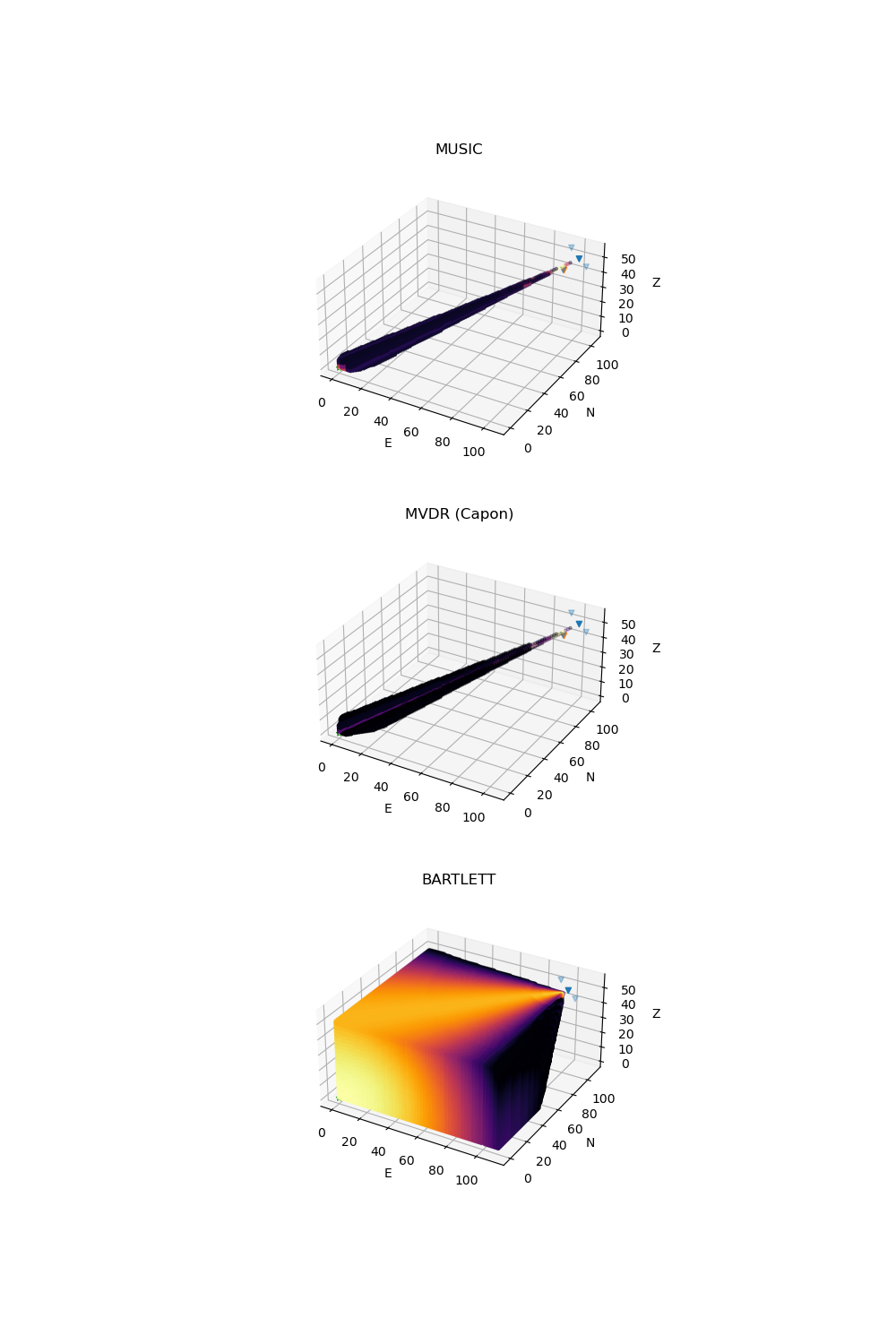
If multiple arrays are available, the beamforming results can be combined (e.g., multiplied) to provide a location.