twistpy.polarization.TimeFrequencyAnalysis6C

class TimeFrequencyAnalysis6C(traN: Trace, traE: Trace, traZ: Trace, rotN: Trace, rotE: Trace, rotZ: Trace, window: dict, dsfacf: int = 1, dsfact: int = 1, frange: Optional[Tuple[float, float]] = None, trange: Optional[Tuple[UTCDateTime, UTCDateTime]] = None, k: float = 1, scaling_velocity: float = 1.0, free_surface: bool = True, verbose: bool = True, timeaxis: str = 'utc')

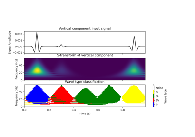
Time-frequency domain six-component polarization analysis.

Single-station six degree-of-freedom polarization analysis on time-frequency decomposed signals. The time-frequency representation is obtained via the S-transform (twistpy.utils.s_transform) [1], [2].

Hint

[1] Sollberger et al. (2018). 6-C polarization analysis using point measurements of translational and rotational ground-motion: theory and applications, Geophysical Journal International, 213(1), https://doi.org/10.1093/gji/ggx542

[2] Sollberger et al. (2020). Seismological processing of six degree-of-freedom ground-motion data, Sensors, 20(23), https://doi.org/10.3390/s20236904

Parameters

traNTrace

North component of translation

traETrace

East component of translation

traZTrace

Vertical component of translation (positive downwards!)

rotNTrace

North component of rotation

rotETrace

East component of rotation

rotZTrace

Vertical component of rotation (right-handed, pointing downwards!)

windowdict

2-D time-frequency window within which the covariance matrices are averaged:

window = {‘number_of_periods’: float, ‘frequency_extent’: float}

The width of the window in time is frequency-dependent and stretches over ‘number_of_periods’ periods, where the period is defined as 1/f. In frequency, the window stretches over the specified ‘frequency_extent’ in Hz.

dsfactint, default=1

Down-sampling factor of the time-axis prior to the computation of polarization attributes.

dsfacfint, default=1

Down-sampling factor of the frequency-axis prior to the computation of polarization attributes.

Warning

Downsampling of the frequency axis (dsfacf > 1) prevents the accurate computation of the inverse S-transform! Down-sampling should be avoided for filtering applications.

frangetuple, (f_min, f_max)

Limit the analysis to the specified frequency band in Hz

trangetuple, (t_min, t_max)

Limit the analysis to the specified time window. t_min and t_max should either be specified as a tuple of two UTCDateTime objects (if timeaxis=’utc’), or as a tuple of float (if timeaxis=’rel’).

kfloat, default=1.

k-value used in the S-transform, corresponding to a scaling factor that controls the number of oscillations in the Gaussian window. When k increases, the frequency resolution increases, with a corresponding loss of time resolution.

See also

twistpy.utils.s_transform

scaling_velocityfloat, default=1.

Scaling velocity (in m/s) to ensure numerical stability. The scaling velocity is applied to the translational data only (amplitudes are divided by scaling velocity) and ensures that both translation and rotation amplitudes are on the same order of magnitude and dimensionless. Ideally, v_scal is close to the S-Wave velocity at the receiver. After applying the scaling velocity, translation and rotation signals amplitudes should be similar.

free_surfacebool, default=True

Specify whether the recording station is located at the free surface in order to use the corresponding polarization models.

verbosebool, default=True

Run in verbose mode.

timeaxis:obj:’str’, default=’utc’

Specify whether the time axis of plots is shown in UTC (timeaxis=’utc’) or in seconds relative to the first sample (timeaxis=’rel’).

Attributes

classificationdict

Dictionary containing the labels of classified wave types at each position of the analysis window in time and frequency. The dictionary has six entries corresponding to classifications for each eigenvector.

classification = {‘0’: list_with_classifications_of_first_eigenvector, ‘1’: list_with_classification_of_second_eigenvector, … , ‘5’: list_with_classification_of_last_eigenvector}

wave_parametersdict

Dictionary containing the estimated wave parameters.

t_pollist of UTCDateTime

Time axis of the computed polarization attributes.

f_polndarray of float

Frequency axis of the computed polarization attributes.

Cndarray of complex128

Complex covariance matrices at each window position

dopndarray of float

Degree of polarization as a function of time- and frequency.

timelist of UTCDateTime

Time axis of the input traces

deltafloat

Sampling interval of the input data in seconds

Methods

classify(svm[, eigenvector_to_classify, ...])	Classify wave types using a support vector machine
filter(svm[, wave_types, ...])	Wavefield separation
plot_classification(ax[, ...])	Plot wave type classification labels as a function of time and frequency.
plot_wave_parameters(...)	Plot estimated wave parameters
polarization_analysis([...])	Perform polarization analysis.
save(name)	Save the current TimeFrequencyAnalaysis6C object to a file on the disk in the current working directory.

Examples using twistpy.polarization.TimeFrequencyAnalysis6C

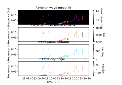
6-C Wave parameter estimation: gulf of alaska earthquake

6-C Wave parameter estimation: gulf of alaska earthquake

6-C wave type fingerprinting

6-C wave type fingerprinting