3-C Polarization analysis and filtering: Real data example using a marsquake recorded by InSight

This example shows the application of TwistPy’s polarization analysis and filtering tools to a marsquake that was recorded by NASA’s InSight Mars lander on mission sol 173. Here, we extract time- and frequency-dependent polarization attributes of the three-component particle motion such as the ellipticity, the degree-of-polarization and the directionality. We then devise a polarization filter to enhance certain phases in the data (in this case, we try to enhance S-phases). The filtering that is demonstrated hereafter has, for example, been used to detect seismic phases that bounce off the Martian core (see Stähler et al., 2021, Seismic detection of the martian core, Science, https://www.science.org/doi/10.1126/science.abi7730).

import matplotlib.pyplot as plt
import numpy as np
from obspy.core import read

from twistpy.polarization import TimeFrequencyAnalysis3C
from twistpy.utils import stransform

# sphinx_gallery_thumbnail_number = 1

We start by reading in the data, which has already been corrected for the instrument response and rotated to a ZNE configuration.

data = read("../example_data/S0173a.mseed")

Now we specify the parameters of the time-frequency window that we use for polarization analysis. The spectral matrices for polarization analysis will be smoothed in a 2D window extending over the number of periods specified by ‘number_of_periods’ and over the frequency range (in Hz) specified by ‘frequency’. Here, we specify a window that is frequency-dependent and extends over a single period in time (1/frequency). In the frequency-direction the window extends over 50 mHz.

window = {"number_of_periods": 5, "frequency_extent": 0.05}

Now we can set up the polarizaiton analysis interface. To compute the S-transform, we use the default value of k=1. (see the example on the S-transform for more information on this parameter).

analysis = TimeFrequencyAnalysis3C(
    N=data[1], E=data[2], Z=data[0], window=window, timeaxis="utc", k=1
)

Computing covariance matrices...
Covariance matrices computed!

To estimate polarization attributes, we use:

analysis.polarization_analysis()

Computing polarization attributes...
Polarization attributes have been computed!

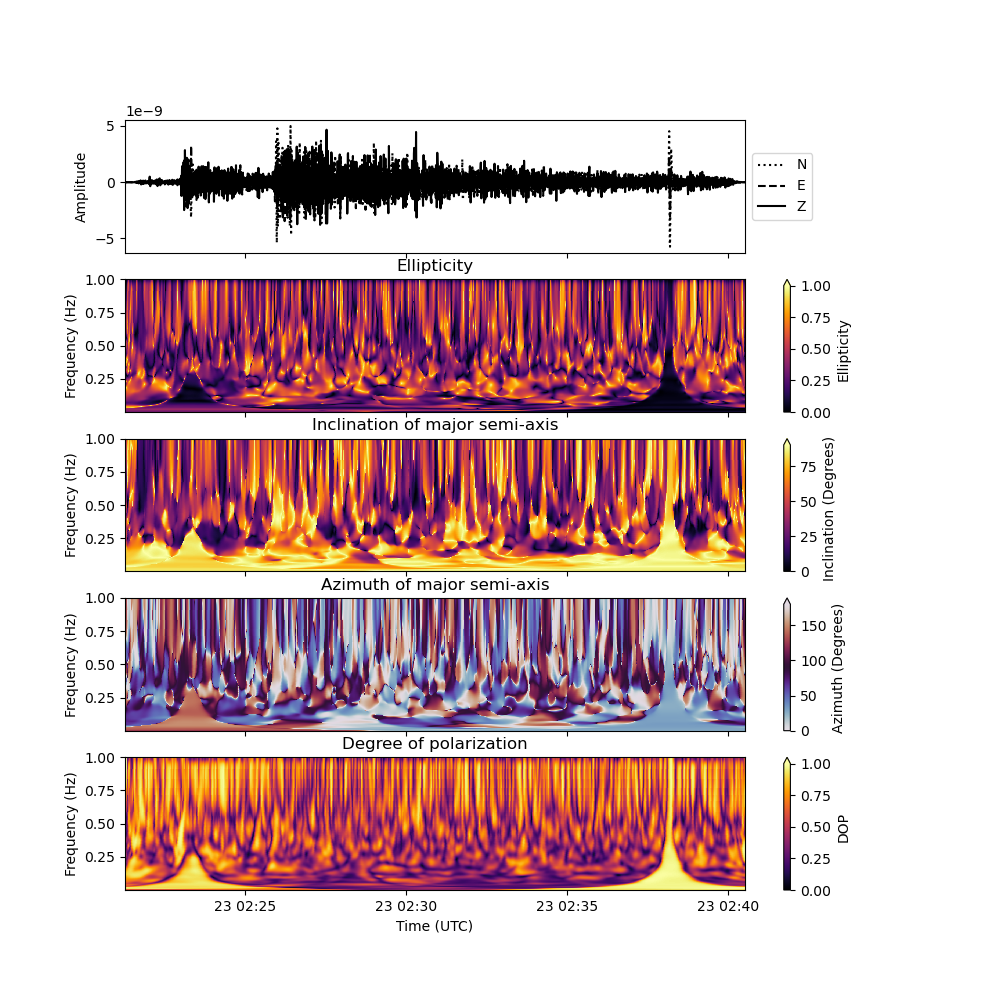
To plot the result, we can make use of the plot_polarization_analysis() method. We want to plot the inclination and azimuth of the major semi-axis of the polarization ellipse and only plot the polarization attributes at time frequency pixels where the signal strength in all three-components exceeds 5 percent of the maximum value:

analysis.plot(major_semi_axis=True, clip=0.00, show=False)

Let us now devise a polarization filter that enhances the S-waves in the signal. For S-waves at close-to- vertical incidence, we would expect the ground to vibrate predominantly in the horizontal direction, we therefore devise a filter that suppresses vertically polarized signals (incidence angle measured from vertical smaller than 60 degrees). Additionally, we only want to keep the part of the signal that is rectilinearly polarized (i.e., the body waves with an ellipticity smaller than 0.4). To automatically generate a plot of the filtered data and the filtered polarization attributes by setting plot_filtered_attributes=True.

data_filtered = analysis.filter(
    elli=[0, 0.4], inc1=[60, 90], plot_filtered_attributes=True, clip=0.0
)

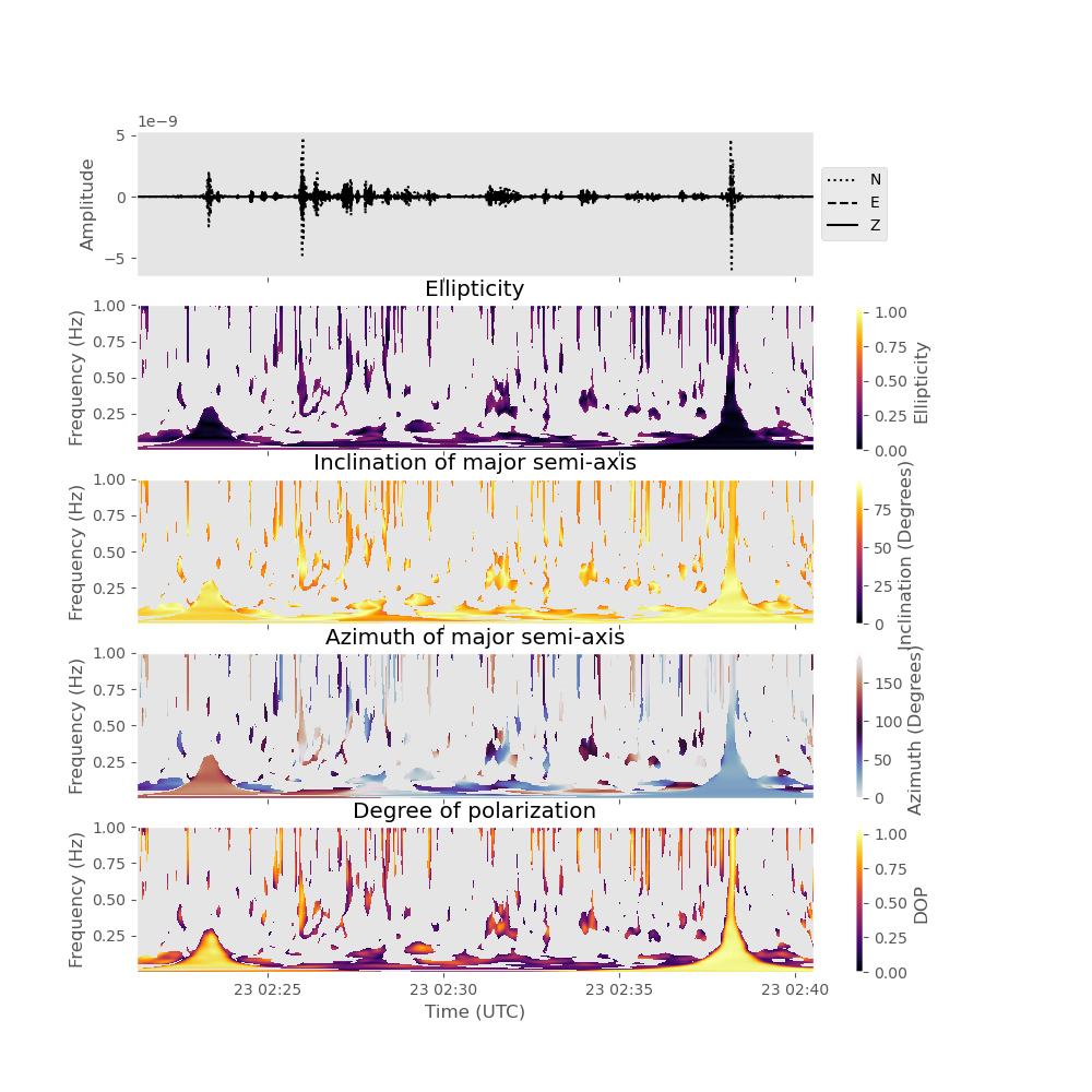
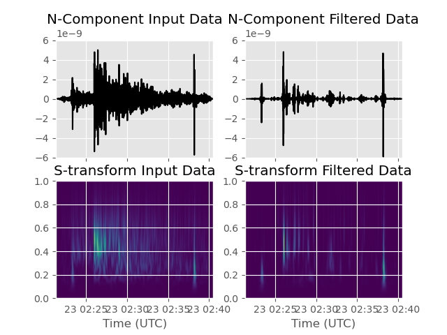
Note that P-wave energy is now widely suppressed, while the S-waves are retained. However, there seems to be a strong horizontally polarized pulse just on top of the P-wave arrival. This pulse corresponds to a data glitch and is not related to the marsquake. Another glitch can be observed at 02:38 UTC. If you look closely, you can see that a horizontally and rectilinearly polarized phase seems to arrive at about 02:31 UTC (about 500 seconds after the P-wave arrival). This phase is interpreted to be an ScS core phase, bouncing off the martian core-mantle boundary (Stähler et al., 2021, Seismic detection of the martian core, Science). Sometimes, it is helpful to plot the time-frequency representation (S-transform) of the signal for interpretation. This can be done in the following way:

# Compute S-transform of North component for plotting
N_stran, f = stransform(data[1].data, k=1)
N_stran_filtered, _ = stransform(
    data_filtered[1].data, k=1
)  # S-transform of filtered data for comparison
plt.style.use("ggplot")

# Plot the result
fig, ax = plt.subplots(2, 2, sharex=True)
ax[0, 0].plot(analysis.t_pol, data[1].data, "k")
ax[0, 0].set_title("N-Component Input Data")
ax[0, 0].set_ylim([-6e-9, 6e-9])
ax[0, 0].xaxis_date()
ax[1, 0].imshow(
    np.abs(N_stran),
    origin="lower",
    aspect="auto",
    extent=[
        analysis.t_pol[0],
        analysis.t_pol[-1],
        analysis.f_pol[0],
        analysis.f_pol[-1],
    ],
)
ax[1, 0].set_xlabel("Time (UTC)")
ax[1, 0].set_title("S-transform Input Data")
ax[1, 0].xaxis_date()

ax[0, 1].plot(analysis.t_pol, data_filtered[1].data, "k")
ax[0, 1].set_title("N-Component Filtered Data")
ax[0, 1].set_ylim([-6e-9, 6e-9])
ax[0, 1].xaxis_date()

ax[1, 1].imshow(
    np.abs(N_stran_filtered),
    origin="lower",
    aspect="auto",
    extent=[
        analysis.t_pol[1],
        analysis.t_pol[-1],
        analysis.f_pol[0],
        analysis.f_pol[-1],
    ],
)
ax[1, 1].set_xlabel("Time (UTC)")
ax[1, 1].set_title("S-transform Filtered Data")
ax[1, 1].xaxis_date()
plt.show()