S-transform

This example illustrates the use of TwistPy’s S-transform functions (twistpy.utils.stransform and twistpy.utils.istransform) to compute a time-frequency representation of a signal and perform some filtering on the time-frequency spectrum.

import matplotlib.pyplot as plt
import numpy as np
from scipy.fft import irfft
from scipy.signal.windows import tukey

from twistpy.utils import stransform, istransform

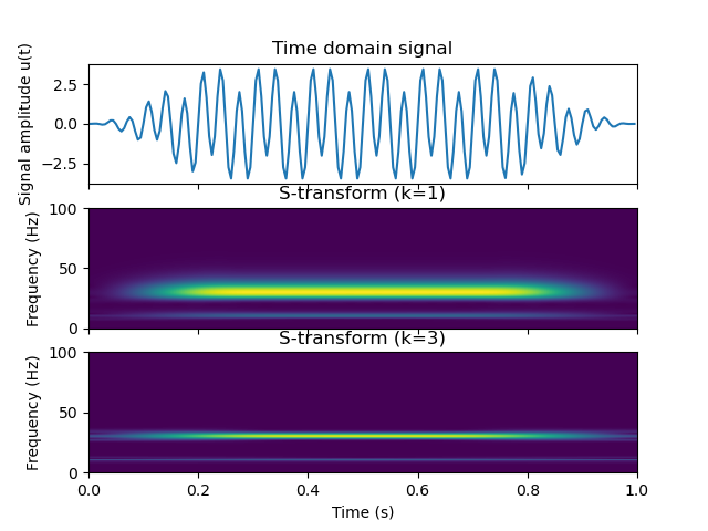
Here, we generate a simple signal consisting of two superimposed sinusoids at 10 and 30 Hz.

dt = 0.005  # Sampling interval (s)
tmin = 0  # Start time of the signal (s)
tmax = 1  # End time of the signal (s)

t = np.arange(tmin, tmax, dt)  # Time axis

f1 = 10  # Frequency of first sinusoid
f2 = 30  # Frequency of second sinusoid

u = np.sin(2 * np.pi * f1 * t) + 3 * np.sin(2 * np.pi * f2 * t)  # Generate signal

taper = tukey(len(t))  # Taper the signal to avoid edge artifacts
u *= taper

The S-transform can be obtained with different k-values as:

u_stran_k1, f = stransform(u, k=1)  # Compute the S-transform with k=1
u_stran_k3, _ = stransform(u, k=3)  # Compute the S-transform with k=3
f_Hz = f / dt  # Convert frequency vector to Hz

figure, axes = plt.subplots(3, 1, sharex=True)
# Plot the time domain signal
axes[0].plot(t, u)
axes[0].set_ylabel("Signal amplitude u(t)")
axes[0].set_title("Time domain signal")

# Plot the magnitude of the S-transform for k=1
axes[1].imshow(
    np.abs(u_stran_k1),
    origin="lower",
    extent=[tmin, tmax, f_Hz[0], f_Hz[-1]],
    aspect="auto",
)
axes[1].set_ylabel("Frequency (Hz)")
axes[1].set_title("S-transform (k=1)")

# Plot the magnitude of the S-transform for k=2
axes[2].imshow(
    np.abs(u_stran_k3),
    origin="lower",
    extent=[tmin, tmax, f_Hz[0], f_Hz[-1]],
    aspect="auto",
)
axes[2].set_xlabel("Time (s)")
axes[2].set_ylabel("Frequency (Hz)")
axes[2].set_title("S-transform (k=3)")

Text(0.5, 1.0, 'S-transform (k=3)')

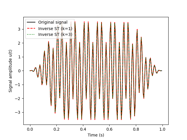
Note that increasing the value of k increases the frequency-resolution. However, this comes at the expense of a lower time-resolution. The inverse S-transform after Schimmel and Gallart (2005, https://doi.org/10.1109/TSP.2005.857065) can now be obtained as:

u_ist_k1 = istransform(u_stran_k1, f)
u_ist_k3 = istransform(u_stran_k3, f, k=3)

plt.figure()
plt.plot(t, u, "k", label="Original signal")
plt.plot(t, u_ist_k1, "r--", label="Inverse ST (k=1)")
plt.plot(t, u_ist_k3, "g:", label="Inverse ST (k=3)")
plt.legend()
plt.xlabel("Time (s)")
plt.ylabel("Signal amplitude u(t)")

Text(44.222222222222214, 0.5, 'Signal amplitude u(t)')

To investigate the effect of time-frequency filtering on the inverse transform, we perform some filtering of the time-frequency decomposed signal. Here, we try to isolate the 10 Hz signal between 0.4 and 0.6 seconds. We then evaluate the differences between the inverse transform after Schimmel and Gallart and the conventional inverse S-transform.

filter_mask_time = np.asarray(
    [0.4, 0.6], dtype="float"
)  # Filter signal between 0.4 and 0.6 s
filter_mask_frequency = np.asarray(
    [5, 15], dtype="float"
)  # Filter signal between 5 and 15 Hz

filter_mask_index = [
    (filter_mask_time / dt).astype("int"),
    (filter_mask_frequency / (f_Hz[1] - f_Hz[0])).astype("int"),
]
filter_mask = np.zeros_like(u_stran_k1)
filter_mask[
    filter_mask_index[1][0]: filter_mask_index[1][1],
    filter_mask_index[0][0]: filter_mask_index[0][1],
] = 1

u_filt_schimmel = istransform(
    u_stran_k1 * filter_mask, f, k=1
)  # Inverse S-transform after Schimmel
u_filt_conventional = irfft(
    np.sum(u_stran_k1 * filter_mask, axis=-1)
)  # Conventional inverse S-transform

fig2, axes2 = plt.subplots(3, 1, sharex=True)
axes2[0].imshow(
    np.abs(u_stran_k1 * filter_mask),
    origin="lower",
    extent=[tmin, tmax, f_Hz[0], f_Hz[-1]],
    aspect="auto",
)
axes2[0].set_ylabel("Frequency (Hz)")
axes2[0].set_title("Filtered S-transform (k=1)")

axes2[1].plot(t, u_filt_schimmel, "k")
axes2[1].set_title("Inverse transform after Schimmel & Gallart (2005)")
axes2[1].set_ylabel("Signal amplitude u(t)")

axes2[2].plot(t, u_filt_conventional, "k")
axes2[2].set_xlabel("Time (s)")
axes2[2].set_ylabel("Signal amplitude u(t)")
axes2[2].set_title("Conventional inverse S-transform")

plt.show()

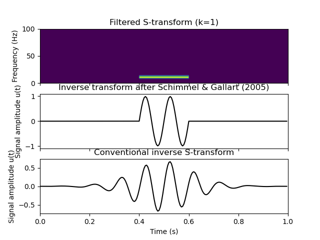
Note that the inverse transform after Schimmel & Gallart provides a better time-localization of the filtered signal compared to the conventional inverse. However, it has to be noted that this inverse transform is only an approximation to the true inverse (the level of approximation is described in Simon, C., Ventosa, S., Schimmel, M., Heldring, A., Dañobeitia, J. J., Gallart, J., & Mànuel, A. 2007. The S-transform and its inverses: Side effects of discretizing and filtering. IEEE Transactions on Signal Processing, 55 (10), 4928–4937. https://doi.org/10.1109/TSP.2007.897893). For filtering purposes, the inverse transform after Schimmel et al. is usually still the better choice.